Journey Through Embeddings: CBOW with negative sampling

The complete code is available as a notebook here.
The weights used in this blog post are stored at this location. They are saved in the same format as used during the training process (cbow_params).

In previous post, we explored the fundamentals of Word2Vec and implemented the Continuous Bag of Words (CBOW) model, which efficiently predicts target words based on their surrounding context. While CBOW is powerful, scaling it to large vocabularies can be computationally challenging due to the softmax function. This is where negative sampling comes in—a clever optimization technique that reduces complexity by focusing only on a few sampled words. In this post, we’ll dive into the intuition behind negative sampling, explore its mechanics through simple examples, and implement it in JAX to make CBOW even more practical for real-world applications.

Introduction

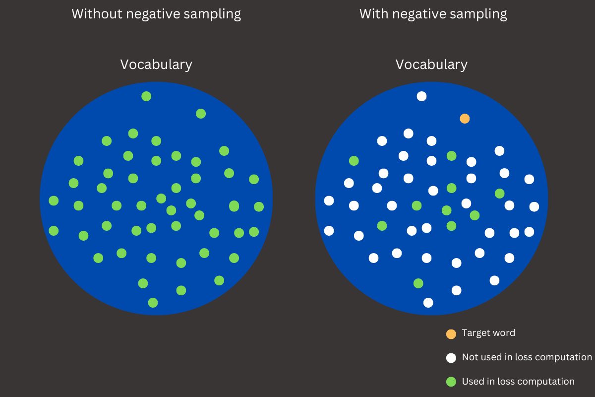
The CBOW (Continuous Bag of Words) model is a powerful approach for learning word embeddings by predicting a target word based on the given context words within a specified window size. However, when working with large datasets, CBOW faces a significant computational challenge due to its reliance on the softmax function. This involves calculating the probability distribution of the target word over the entire vocabulary, a process that becomes increasingly resource-intensive as the vocabulary size grows.

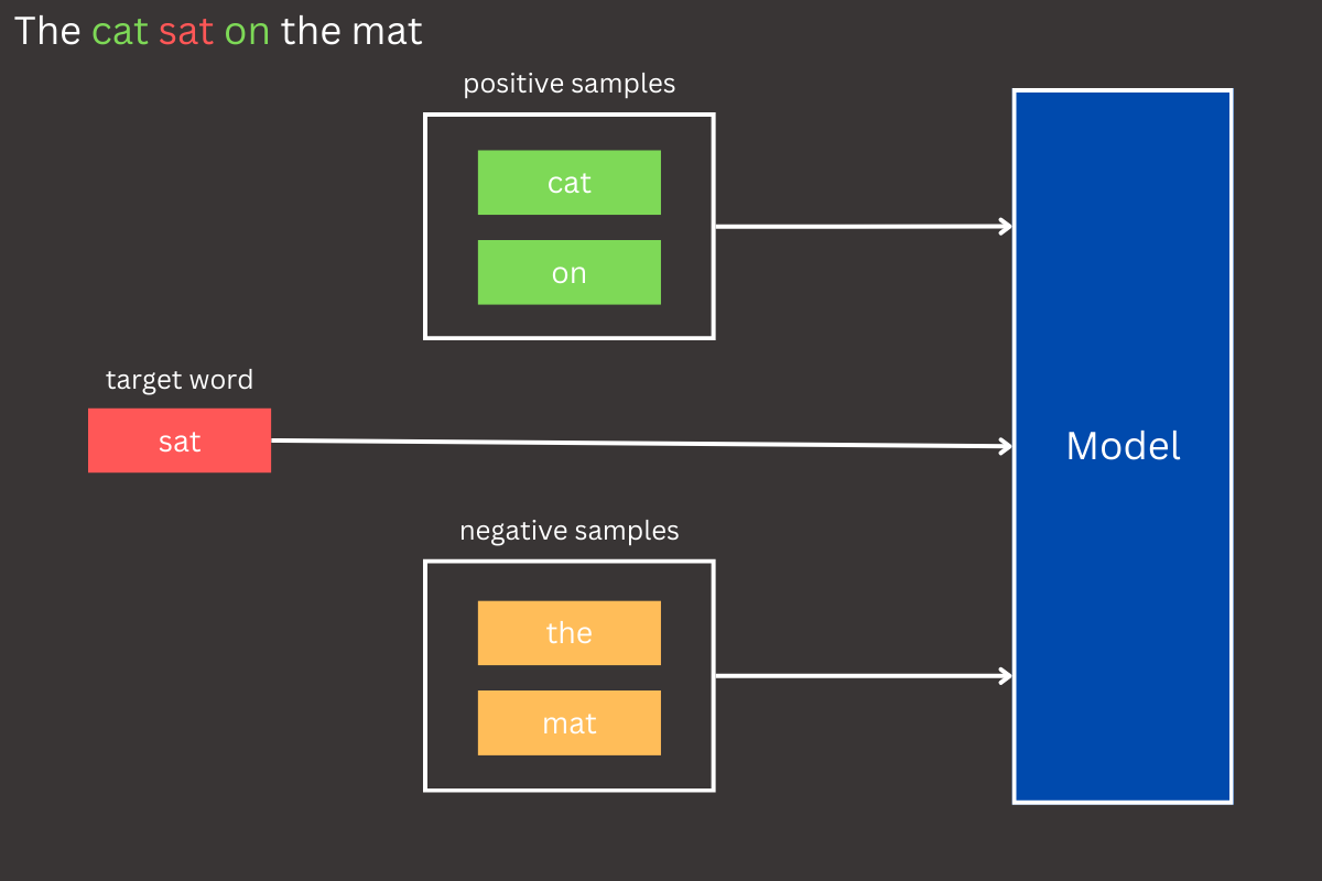
To address this issue, negative sampling is introduced as an optimization technique. Instead of computing probabilities for all words in the vocabulary, negative sampling simplifies the process by focusing only on the target word and a small, randomly selected subset of words (negative samples). The model learns to distinguish between the correct target word and these randomly chosen negatives, significantly reducing computational overhead while retaining the quality of the embeddings. This approach not only accelerates training but also makes the CBOW model scalable to large corpora. For example, if the context is The cat is on the and the target word is mat, the model would update its embeddings to increase the similarity to mat while reducing similarity to unrelated words like pizza or river. This greatly reduces computational complexity while preserving embedding quality.

Let’s explore the inner workings of how negative sampling can be integrated into the CBOW model and the key changes it brings to the training process.

Learning with negative sampling

While we’ve already mentioned how negative sampling addresses the challenges of softmax computation, let’s dive deeper and compare it with an implementation where softmax is used to obtain the vocabulary probability distribution

@jax.jit
def loss_fn(params, context_vector, target):
    logits = forward(params, context_vector)  # (BATCH_SIZE, VOCAB_SIZE)

    # compute the loss
    target_ohe = jnn.one_hot(target, len(vocabulary)) # (BATCH_SIZE, VOCAB_SIZE)
    loss_result = optax.losses.softmax_cross_entropy(logits, target_ohe).mean() # (BATCH_SIZE,)

    return loss_result

The loss_fn function in our implementation illustrates this process. It calculates the cross-entropy loss between the predicted probabilities and the one-hot encoded target word using optax.losses.softmax_cross_entropy.

While effective for smaller vocabularies, this approach becomes computationally expensive for large datasets. The softmax function requires calculating the probability of the target word against every other word in the vocabulary, leading to significant overhead as the vocabulary size grows.

Let’s dive into the loss function and understand it from a mathematical perspective. The loss function for negative sampling aims to distinguish the correct target word (positive example) from randomly selected words (negative samples). It’s important to note that the negative samples must be words that do not match the target word. Mathematically, the loss function is defined as:

• w_target: the target word (positive example)
• w_i : negative samples (word randomly chosen from the vocabulary)
• v_c : the context vector (averated embeddings of context words)
• W[.]: represents embeddings from the output layer (target/negative word embeddings)
• k: number of negative samples
• σ: represents sigmoid function

Number of negative samples k, generated for each positive sample, is a hyperparameter that must be defined before the learning process begins. The choice of k directly affects both the computational efficiency and the quality of the learned embeddings.

• A small  k  (e.g., 5–10) is often sufficient for smaller datasets and works well when the vocabulary is limited. It reduces computational cost but may result in slightly less precise embeddings
• A larger  k  (e.g., 15–20 or more) can improve embedding quality for larger datasets with extensive vocabularies, but it comes at the cost of increased computation per iteration

In practice, common choices of k depend on the size of the dataset and vocabulary. For example, the original Word2Vec implementation uses k = 5–10 for smaller tasks and k=15–20 for larger corpora. Finding the right balance is essential, as too many negative samples can unnecessarily slow training without significant benefits, while too few may result in suboptimal embeddings.

For a positive component, we analyze its contribution to the loss function. The model calculates the dot product between the context vector v_c and the embedding of the target word u[w_target]. This result is then passed through a sigmoid function σ, which maps the output to a probability between 0 and 1. This probability reflects the likelihood of the correct target word given the context, and the model optimizes to maximize this value.

For a negative component, the model computes a value for each of the  k  negative samples w_i by taking the dot product between the embedding of the negative sample word and the context vector, then multiplying the result by -1. This dot product is then passed through a sigmoid function σ, which maps it to a probability between 0 and 1. The multiplication by -1 ensures that the model minimizes the similarity between the context vector and the negative samples, effectively minimizing their contribution to the predicted probability.

Implementation

Now, let’s build on what we’ve learned about negative sampling. Unlike the approach discussed in the previous blog post, we must address the generation of negative samples for each positive sample in our dataset. To achieve this, we’ll introduce a new function, generate_training_text_with_negative_samples(…), which extends the previous implementation by adding two key arguments

• number_of_negatives: Specifies how many negative samples to generate per positive sample
• token_probabilities: Represents the probability distribution of tokens in the dataset, used to sample negative examples more effectively
  • By leveraging the token probabilities, we can ensure the selection process reflects the dataset’s distribution, enhancing the model’s ability to differentiate contextually relevant words from irrelevant ones

def generate_training_text_w_negative_samples(
        tokens: list[str],
        vocabulary: dict[str, int],
        window_size: int = 2,
        stride: int = 1,
        batch_size: int | None = None,
        to_ids: bool = False,
        number_of_negatives: int | None = 5,
        token_probabilities: np.ndarray | None = None
):
    len_tokens = len(tokens)
    range_len = len(range(window_size + 1, len_tokens - window_size - 1, stride))

    negative_samples_generated = None
    if number_of_negatives:
        negative_samples_generated = np.random.choice(
            list(vocabulary.keys()),
            size=(range_len, number_of_negatives),
            p=token_probabilities
        )

    batch_context, batch_positives, batch_negatives = [], [], []
    for token_idx in range(window_size + 1, len_tokens - window_size - 1, stride):
        left_context = tokens[token_idx - window_size:token_idx]
        right_context = tokens[token_idx + 1:token_idx + window_size + 1]

        negative_samples = []
        if number_of_negatives:
            negative_samples = negative_samples_generated[token_idx - window_size - 1, :] if negative_samples_generated is not None else []

            while tokens[token_idx] in negative_samples:
                negative_samples = np.random.choice(
                    list(vocabulary.keys()),
                    size=(number_of_negatives, ),
                    p=token_probabilities
                )

        if to_ids:
            left_context_vector = [vocabulary.get(word, vocabulary["<unk>"]) for word in left_context]
            right_context_vector = [vocabulary.get(word, vocabulary["<unk>"]) for word in right_context]
            target_vector = vocabulary.get(tokens[token_idx], vocabulary["<unk>"])

            context_vector = left_context_vector + right_context_vector
            negative_samples_vector = [vocabulary.get(word, vocabulary["<unk>"]) for word in negative_samples]
        else:
            left_context_vector = left_context
            right_context_vector = right_context
            target_vector = tokens[token_idx]

            context_vector = left_context_vector + right_context_vector
            negative_samples_vector = negative_samples

        if target_vector == vocabulary["<unk>"]:
            continue

        if batch_size is None:
            yield context_vector, [target_vector, ], negative_samples_vector
        else:
            batch_context.append(context_vector)
            batch_positives.append(target_vector)
            batch_negatives.append(negative_samples_vector)

            if len(batch_positives) == batch_size:
                yield np.array(batch_context), np.array(batch_positives), np.array(batch_negatives)
                batch_context, batch_positives, batch_negatives = [], [], []

    if len(batch_positives) > 0 or len(batch_context) > 0 or len(batch_negatives) > 0:
        yield np.array(batch_context), np.array(batch_positives), np.array(batch_negatives)
                

This implementation may not be the most optimal solution among all possible approaches, but it is sufficient for our needs. A notable feature of this implementation is the use of a random generator to produce negative samples for each positive example in the dataset (lines 14-20). These generated samples are temporarily stored in a variable and later retrieved within a for-loop, where they are paired as target and context words and added to the batch array. Once the batch array reaches the desired size (batch_size), it is yielded from the function, ready for training.

To generate negative samples, token probabilities are computed based on word frequencies in the dataset. Each word’s count is raised to the power of 0.75 to downweight very frequent words and balance the contribution of less frequent ones. The smoothed probabilities are then normalized to ensure they sum up to 1, creating a valid probability distribution for sampling.

# compute the token probabilities
token_probabilities = {
    word: train_token_counter[word] ** 0.75 if word in train_token_counter else 0
    for word in vocabulary.keys()
}
smoothed_token_probabilities = np.array([token_probabilities[word] for word in vocabulary.keys()])
total_smoothed_sum = np.sum(smoothed_token_probabilities)

negative_sampling_probabilities = smoothed_token_probabilities / total_smoothed_sum


NEGATIVE_SAMPLES_COUNT = 10
WINDOWS_SIZE = 10
        
for (context_vector, target_vector, negative_samples) in generate_training_text_w_negative_samples(train, vocabulary, window_size=WINDOWS_SIZE, stride=1, batch_size=2, to_ids=False, number_of_negatives=NEGATIVE_SAMPLES_COUNT, token_probabilities=negative_sampling_probabilities):
    print(f"Context vectors: {context_vector}")
    print(f"Target vectors: {target_vector}")
    print(f"Negative samples: {negative_samples}")
    
    break


Context vectors: [['authority' 'rejects' 'hierarchy' 'anarchism' 'calls' 'abolition'
  'holds' 'unnecessary' 'harmful' 'leftwing' 'spectrum' 'libertarian'
  'libertarian' 'wing' 'libertarian' 'socialism' 'socialist' 'strong'
  'socialism' 'humans']
 ['rejects' 'hierarchy' 'anarchism' 'calls' 'abolition' 'holds'
  'unnecessary' 'harmful' 'leftwing' 'placed' 'libertarian' 'libertarian'
  'wing' 'libertarian' 'socialism' 'socialist' 'strong' 'socialism'
  'humans' 'lived']]
Target vectors: ['placed' 'spectrum']
Negative samples: [['preface' 'capita' 'taught' 'cartesian' 'commercial' 'felt'
  'institutional' 'project' 'economics' 'turning']
 ['new' '1850' 'comedian' 'capital' 'pink' 'worker' 'glory' 'angel'
  'sister' 'background']]
  
  
  
for (context_vector, target_vector, negative_samples) in generate_training_text_w_negative_samples(train, vocabulary, window_size=WINDOWS_SIZE, stride=1, batch_size=2, to_ids=True, number_of_negatives=NEGATIVE_SAMPLES_COUNT, token_probabilities=negative_sampling_probabilities):
    print(f"Context vectors: {context_vector}")
    print(f"Target vectors: {target_vector}")
    print(f"Negative samples: {negative_samples}")
    
    break
    

Context vectors: [[ 674 9644 4454 5451 2647 6465 2018 9885 8076 8680 2578 7284 7284 2484
  7284 4195 1933  528 4195 1003]
 [9644 4454 5451 2647 6465 2018 9885 8076 8680  839 7284 7284 2484 7284
  4195 1933  528 4195 1003 1214]]
Target vectors: [ 839 2578]
Negative samples: [[ 458  583 5046 4606 7396 8626 1689 5517 6424 8616]
 [4733 9775 3266 3849  743 7907 3883  598 1313 4064]]      

At this point, the implementation of CBOW with negative sampling should be more straightforward to understand. The plan is to develop two functions: one to compute the positive logits and another to compute the negative logits. These will then be integrated into the loss function, as described in Figure 3.

The initialization in JAX will remain the same as in the CBOW model implementation. We will define the embedding dimension, which represents the number of features in the word embedding vector. This dimension is used to initialize the embedding matrix  W , with a shape of  VOCABULARY_SIZE x EMBEDDING_DIMENSION. This matrix will store the embeddings for all words in the vocabulary.

EMBEDDING_DIM = 300

embedding_init = jax.nn.initializers.glorot_uniform()

cbow_params = {
    "embedding": embedding_init(jax.random.PRNGKey(69), (len(vocabulary), EMBEDDING_DIM))
}

@jax.jit
def context_projection(params, context_samples):
    context_vector_state = params["embedding"][context_samples]

    return jnp.mean(context_vector_state, axis=1)  # (BATCH, EMBEDDING_DIM)
    
    
    
@jax.jit
def positive_forward(params, context_vector, target_vector):
    context_projection_result = context_projection(params, context_vector) # (BATCH_SIZE, EMBEDDING_DIM)
    target_embeddings = params["embedding"][target_vector] # (BATCH_SIZE, EMBEDDING_DIM)

    positive_scores = jnp.einsum("bd,bd->b", context_projection_result, target_embeddings) # (BATCH_SIZE,)

    return positive_scores # (BATCH_SIZE,)    

The positive_forward(…) (line 17-24) function is similar in structure to the previously implemented forward function, but it is specifically designed to compute the positive logits for the loss function in the context of negative sampling. The key difference is that, instead of computing logits for the entire vocabulary, this function focuses only on the dot product between the averaged context vector and the embeddings of the target words. This design aligns with the requirements of the loss function. Let’s break it down:

• Averaged context vector
  • The function begins by calculating the averaged context vector using the context_projection function, which produces context_projection_result with a shape of  (BATCH_SIZE, EMBEDDING_DIMENSION)
  • This represents the average of the embeddings for all context words in each sample of the batch
• Target embeddings
  • The embeddings for the target words are retrieved from the embedding matrix (line 20) using provided indices inside target_vector
  • target_embeddings has the same shape as the context projection: (BATCH_SIZE, EMBEDDING_DIMENSION)
• Dot product
  • To compute the positive scores (or logits) the function calculates the dot product between the averated context vector and the corresponding target embeddings for each sample in the batch
  • This operation is performed with line 22
    • The jnp.einsum function is a versatile tool that simplifies various operations, including reductions, dot products, element-wise products, and tensor reordering, making it highly efficient for mathematical computations
  • Resulting positive_scores (line 22) has a shape of (BATCH_SIZE, ) where each element represents score for the corresponding sample in the batch

for (context_vector, target_vector, negative_samples) in generate_training_text_w_negative_samples(train, vocabulary, window_size=WINDOWS_SIZE, stride=1, batch_size=2, to_ids=True, number_of_negatives=NEGATIVE_SAMPLES_COUNT, token_probabilities=negative_sampling_probabilities):
    print(f"Context vectors: {context_vector}")
    print(f"Target vectors: {target_vector}")
    print(f"Negative samples: {negative_samples}")
    
    break
    
Context vectors: [[ 674 9644 4454 5451 2647 6465 2018 9885 8076 8680 2578 7284 7284 2484
  7284 4195 1933  528 4195 1003]
 [9644 4454 5451 2647 6465 2018 9885 8076 8680  839 7284 7284 2484 7284
  4195 1933  528 4195 1003 1214]]
Target vectors: [ 839 2578]
Negative samples: [[7111  889 8682  239 7112  957  781 3557   70 1005]
 [ 109 6872 1468 1153 6224 1087 3074 1742 2390   22]]


positive_forward(cbow_params, context_vector, target_vector)

Array([0.00246207, 0.00050519], dtype=float32)    

The function for calculating negative logits (or scores) has a structure similar to the one used for positive logits, with the key difference being that the embeddings for negative samples include an additional dimension to account for multiple negative samples per target word. This extra dimension is handled using jnp.einsum, which efficiently computes the dot product between the averaged context vector and the embeddings for each negative sample across the batch. This ensures that the output captures the scores for all negative samples, resulting in a shape of (BATCH_SIZE, NEGATIVE_SAMPLES).

EMBEDDING_DIM = 300

embedding_init = jax.nn.initializers.glorot_uniform()

cbow_params = {
    "embedding": embedding_init(jax.random.PRNGKey(69), (len(vocabulary), EMBEDDING_DIM))
}

@jax.jit
def context_projection(params, context_samples):
    context_vector_state = params["embedding"][context_samples]

    return jnp.mean(context_vector_state, axis=1)  # (BATCH, EMBEDDING_DIM)
    
    
    
@jax.jit
def positive_forward(params, context_vector, target_vector):
    context_projection_result = context_projection(params, context_vector) # (BATCH_SIZE, EMBEDDING_DIM)
    target_embeddings = params["embedding"][target_vector] # (BATCH_SIZE, EMBEDDING_DIM)

    positive_scores = jnp.einsum("bd,bd->b", context_projection_result, target_embeddings) # (BATCH_SIZE,)

    return positive_scores # (BATCH_SIZE,)    
    
    
@jax.jit
def negative_forward(params, context_vector, negative_vector):
    context_projection_result = context_projection(params, context_vector) # (BATCH_SIZE, EMBEDDING_DIM)
    negative_target_embeddings = params["embedding"][negative_vector] # (BATCH_SIZE, NEGATIVE_SAMPLES, EMBEDDING_DIM)

    negative_scores = jnp.einsum("bd,bnd->bn", context_projection_result, negative_target_embeddings) # (BATCH_SIZE, NEGATIVE_SAMPLES)

    return negative_scores # (BATCH_SIZE, NEGATIVE_SAMPLES)

• Averaged context vector
  • The averaged context vector is computed using context_projection, resulting in a shape of (BATCH_SIZE, EMBEDDING_DIM)
• Negative sample embeddings
  • The embeddings for the negative samples are retrieved from the embedding matrix using negative_vector. The shape is  (BATCH_SIZE, NEGATIVE_SAMPLES, EMBEDDING_DIM) 
• Dot product
  • The dot product between the context vector and the embeddings of the negative samples is computed using jnp.einsum. This results in negative_scores with shape (BATCH_SIZE, NEGATIVE_SAMPLES) , where each entry represents the score for a specific negative sample in the batch
  • jnp.einsum(“bd,bnd->bn”, context_projection_result, negative_target_embeddings)
    • This line computes the dot product between the averaged context vector and each negative sample’s embedding
      • bd represents batch dimension (b) and embedding dimension (d)
      • bnd represents the batch dimension (b), number of negative samples (n) and embedding dimension (d) of the negative sample embeddings
      • bn specify the output shape, reducing the embedding dimension (d) by performing a dot product for each negative sample in the batch
    • einsum provides an elegant and concise way to perform this operation, avoiding the need for additional functions like vmap or multiple dot calls that would typically be required to handle such batch-wise computations

for (context_vector, target_vector, negative_samples) in generate_training_text_w_negative_samples(train, vocabulary, window_size=WINDOWS_SIZE, stride=1, batch_size=2, to_ids=True, number_of_negatives=NEGATIVE_SAMPLES_COUNT, token_probabilities=negative_sampling_probabilities):
    print(f"Context vectors: {context_vector}")
    print(f"Target vectors: {target_vector}")
    print(f"Negative samples: {negative_samples}")
    
    break
    
    
negative_forward(cbow_params, context_vector, negative_samples)

Array([[-1.7337849e-03,  7.4543175e-05,  1.8398713e-03,  9.0001291e-04,
         8.2156190e-04,  1.2978809e-03, -3.0007656e-04, -2.2598097e-04,
         9.9722994e-04,  6.9780531e-04],
       [ 8.9381385e-04,  1.5331763e-03,  9.7417342e-04, -8.8747730e-04,
        -5.6410453e-04, -7.9983805e-04,  3.7086254e-05,  1.1828387e-03,
         6.6665921e-04, -1.3335008e-04]], dtype=float32)
         
negative_forward(cbow_params, context_vector, negative_samples).shape

(2, 10)             

EMBEDDING_DIM = 300

embedding_init = jax.nn.initializers.glorot_uniform()

cbow_params = {
    "embedding": embedding_init(jax.random.PRNGKey(69), (len(vocabulary), EMBEDDING_DIM))
}

@jax.jit
def context_projection(params, context_samples):
    context_vector_state = params["embedding"][context_samples]

    return jnp.mean(context_vector_state, axis=1)  # (BATCH, EMBEDDING_DIM)


@jax.jit
def positive_forward(params, context_vector, target_vector):
    context_projection_result = context_projection(params, context_vector) # (BATCH_SIZE, EMBEDDING_DIM)
    target_embeddings = params["embedding"][target_vector] # (BATCH_SIZE, EMBEDDING_DIM)

    positive_scores = jnp.einsum("bd,bd->b", context_projection_result, target_embeddings) # (BATCH_SIZE,)

    return positive_scores # (BATCH_SIZE,)

@jax.jit
def negative_forward(params, context_vector, negative_vector):
    context_projection_result = context_projection(params, context_vector) # (BATCH_SIZE, EMBEDDING_DIM)
    negative_target_embeddings = params["embedding"][negative_vector] # (BATCH_SIZE, NEGATIVE_SAMPLES, EMBEDDING_DIM)

    negative_scores = jnp.einsum("bd,bnd->bn", context_projection_result, negative_target_embeddings) # (BATCH_SIZE, NEGATIVE_SAMPLES)

    return negative_scores # (BATCH_SIZE, NEGATIVE_SAMPLES)

@jax.jit
def loss_fn(params, context_vector, negative_target, positive_target):
    positive_logits = positive_forward(params, context_vector, positive_target)  # (BATCH_SIZE,)
    negative_logits = negative_forward(params, context_vector, negative_target)  # (BATCH_SIZE, NUM_NEGATIVE_SAMPLES)

    all_logits = jnp.concatenate([positive_logits[:, None], -negative_logits], axis=1)  # (BATCH_SIZE, NUM_NEGATIVE_SAMPLES + 1)
    all_loss = -jnn.log_sigmoid(all_logits)  # (BATCH_SIZE, NUM_NEGATIVE_SAMPLES + 1)

    positive_loss = jnp.mean(all_loss[:, 0])
    negative_loss = jnp.mean(all_loss[:, 1:].sum(axis=1))

    return positive_loss + negative_loss, (positive_loss, negative_loss)

For the loss function, we only need the indices for the context words, negative samples, and target words as arguments. Using these, we call the positive_forward and negative_forward functions to compute the scores (or logits). These outputs are referred to as logits because no final transformation, such as sigmoid or softmax, has been applied after the dot product. Logits represent raw, untransformed values that are later processed by functions like sigmoid or softmax during loss computation.

for (context_vector, target_vector, negative_samples) in generate_training_text_w_negative_samples(train, vocabulary, window_size=WINDOWS_SIZE, stride=1, batch_size=2, to_ids=True, number_of_negatives=NEGATIVE_SAMPLES_COUNT, token_probabilities=negative_sampling_probabilities):
    print(f"Context vectors: {context_vector}")
    print(f"Target vectors: {target_vector}")
    print(f"Negative samples: {negative_samples}")
    break
    
    
loss_fn(cbow_params, context_vector, negative_samples, target_vector)  

(Array(7.6256967, dtype=float32),
 (Array(0.69240576, dtype=float32), Array(6.933291, dtype=float32)))  

Training

With this, the core implementation is complete. All that’s left is to define the training loop, and we’ll be ready to train the CBOW model using the negative sampling method.

print("Generating full dataset")

full_dataset = list(generate_training_text_w_negative_samples(train, vocabulary, window_size=WINDOWS_SIZE, stride=STRIDE, batch_size=BATCH_SIZE, to_ids=True, number_of_negatives=NEGATIVE_SAMPLES_COUNT, token_probabilities=negative_sampling_probabilities, shuffle=True))


LR = 1e-3
EPOCHS = 10

optimizer = optax.adam(learning_rate=LR)
opt_state = optimizer.init(cbow_params)

training_loss = []
training_positive_loss, training_negative_loss = [], []



with tqdm() as training_progress:
    for epoch_id in range(EPOCHS):
        training_progress.set_description(f"Training: Epoch {epoch_id + 1}/{EPOCHS}")
        training_progress.reset(total=len(full_dataset))

        training_epoch_loss = []
        training_epoch_positive_loss, training_epoch_negative_loss = [], []
        for (context_vector, target_vector, negative_samples) in full_dataset:
            context_vector, target_vector, negative_samples = shuffle_batch(context_vector, target_vector, negative_samples)
            
            (value_of_loss, pos_neg_loss), grads = jax.value_and_grad(loss_fn, has_aux=True)(cbow_params, context_vector, negative_samples, target_vector)
            updates, opt_state = optimizer.update(grads, opt_state)
            cbow_params = optax.apply_updates(cbow_params, updates)

            training_epoch_loss.append(value_of_loss)
            training_epoch_positive_loss.append(pos_neg_loss[0])
            training_epoch_negative_loss.append(pos_neg_loss[1])

            training_progress.set_postfix({"loss": value_of_loss})
            training_progress.update(1)

        training_loss.append(np.mean(training_epoch_loss))
        training_positive_loss.append(np.mean(training_epoch_positive_loss))
        training_negative_loss.append(np.mean(training_epoch_negative_loss))

Finally, we can use the same approach from our original CBOW implementation to find similar words and solve word analogies using the trained embeddings. For hyperparameters, we will adopt a similar set of values used in the previous post for training the CBOW model:

• TOP_K_ARTICLES
  • Defines the number of articles loaded from Wikipedia using the Hugging Face datasets library
  • Value: 50000
• TOP_K
  • Specifies the number of tokens retained in the vocabulary after filtering
  • Value: 30000
• WINDOW_SIZE
  • Determines the number of context words to include on each side of the target word
  • Value: 10
• EMBEDDING_DIM
  • Sets the dimensionality of the embedding vectors in the embedding matrix
  • Value: 300
• BATCH_SIZE
  • Defines the number of samples included in each training batch
  • Value: 2048
• LR (learning rate)
  • Controls the step size for weight updates during optimization
  • Value: 1e-3
• EPOCHS
  • Specifies the number of complete passes through the training data
  • Value: 25 epochs
• NEGATIVE_SAMPLES_COUNT
  • Specifies the number of negative samples per positive sample
  • Value: 5

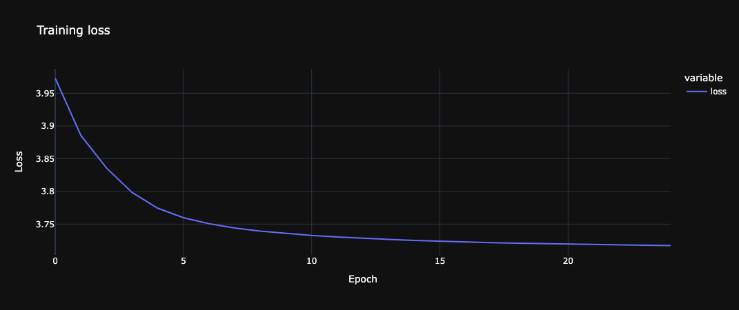
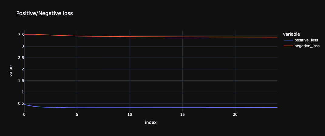
Figures 4 and 5 illustrate the loss during the training process. Figure 4 presents the global loss values, while Figure 5 breaks it down into the two components contributing to the global loss. Intuitively, both loss components are expected to decrease over time and across epochs. However, the exact values depend on several factors, including the dataset size, batch size, number of negative samples, learning rate, and the duration of the training process.

All the operations used in the CBOW model implementation can be applied here as well. For reference, I recommend revisiting the blog post on the CBOW model and exploring the code sample available on GitHub.

Next steps

The best way to solidify your understanding of word embeddings is to experiment further. Try training your own models on different datasets, tweaking hyperparameters, and analyzing the resulting embeddings. Explore different visualization techniques, such as t-SNE, to gain a more intuitive grasp of how the model captures semantic relationships. By actively engaging with the material and pushing the boundaries of what you’ve learned, you’ll develop a deeper appreciation for the power and potential of word embeddings.

Summary

This blog post explored the concept of word embeddings, focusing on the Continuous Bag-of-Words (CBOW) model with negative sampling. We learned how CBOW predicts a target word from its surrounding context and how negative sampling improves training efficiency. A practical Python implementation demonstrated the steps involved in building and training a simple CBOW model, providing a hands-on understanding of these powerful techniques used in natural language processing.

The complete code is available as a notebook here.
The weights used in this blog post are stored at this location. They are saved in the same format as used during the training process (cbow_params).