Journey Through Embeddings: Word2vec CBOW

The complete code is available as a notebook here.
The weights used in this blog post are stored at this location. They are saved in the same format as used during the training process (cbow_params).

Word embeddings have revolutionized natural language processing by transforming text into meaningful numerical representations that capture the relationships between words. In this blog, we focus on Word2Vec, a foundational technique in embedding methods, with a particular emphasis on the Continuous Bag of Words (CBOW) model. CBOW learns embeddings by predicting a target word from its surrounding context, capturing word similarity based on their positions and relationships within the text. We’ll explore its architecture, how it works, and why it remains a crucial method for understanding linguistic patterns. Additionally, we’ll implement the CBOW model step by step using Python and JAX, showcasing how modern tools can bring this classic technique to life. Whether you’re new to word embeddings or revisiting this classic method, this post will guide you through the inner workings of CBOW in a practical and hands-on way. The complete code is available as a notebook here.

Introduction

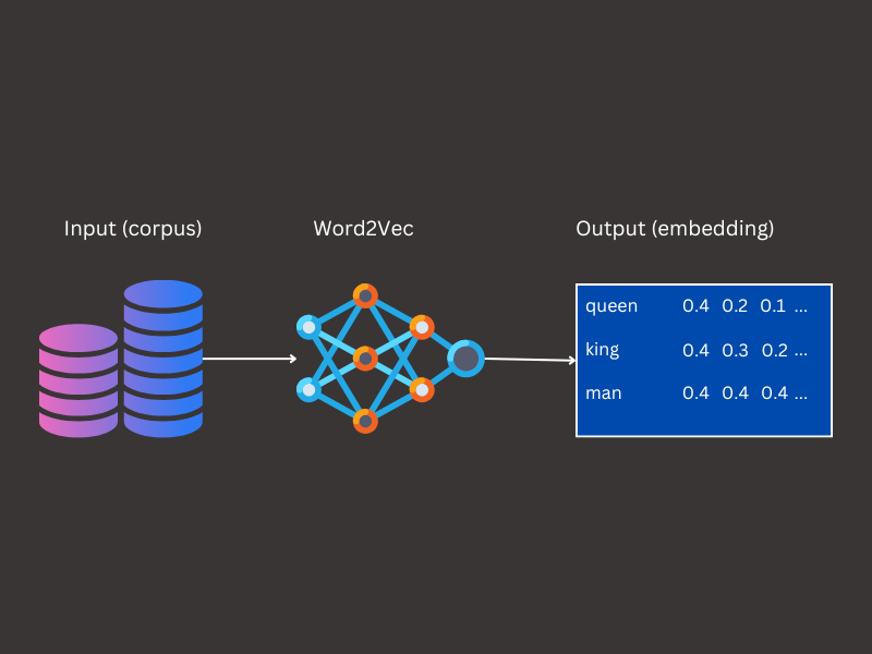
Imagine trying to teach a computer the relationship between words like king, queen, man, and woman. Humans understand that king and queen are related, just as man and woman are, but traditional methods like word counting or assigning unique IDs to words can’t capture these deeper connections. This is where Word2Vec comes in. Word2Vec is a technique for representing words as vectors of numbers, where similar words have similar vectors. For example:

• King and Queen might have vectors close to each other because they share similar roles
• The difference between Paris and France could be similar to the difference between Berlin and Germany.

Word2Vec achieves this by analyzing massive amounts of text to learn relationships based on how words appear together. If coffee often appears near cup or morning, their vectors will be close, reflecting their semantic similarity. Beyond just identifying similar words, Word2Vec can solve analogies like:

king – man + women = queen

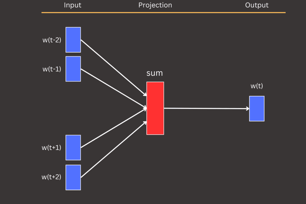
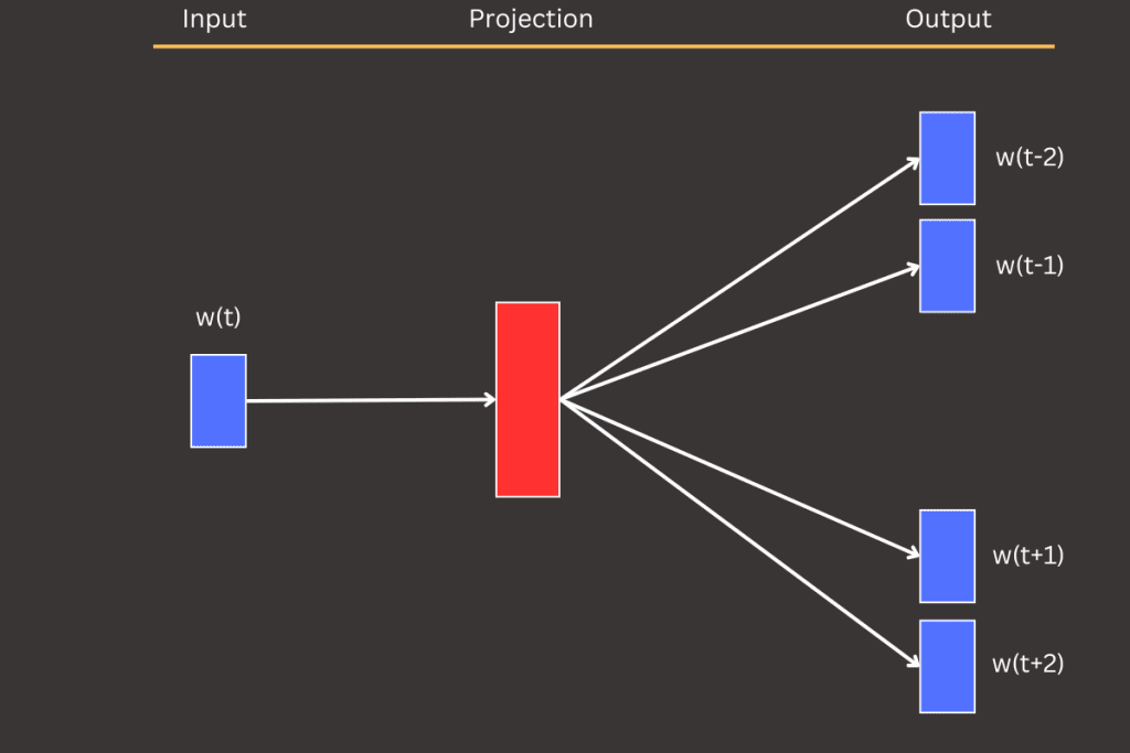
Word2Vec introduces two main model types: Continuous Bag of Words (CBOW) and Skip-gram. CBOW predicts a target word based on its surrounding context, while Skip-gram works in reverse, predicting context words from a given target word. In this blog post, we’ll focus on CBOW and explore its architecture, implementation, and applications.

Word2Vec wasn’t just a breakthrough on its own—it became the spark for more powerful models like large language models (LLMs) used today. By introducing ideas like word embeddings and context-based learning, Word2Vec laid the groundwork for modern architectures, from GPT to BERT, that take these concepts to the next level. It’s where the journey toward understanding language computationally truly began.

Word2Vec internals

Word2Vec derives its power from learning meaningful word embeddings by analyzing relationships between words in text. It processes massive text datasets by breaking them into smaller pieces, such as sentences or phrases. For each piece, it identifies word relationships based on their co-occurrence within a fixed window size. The window size defines how many words on either side of the target word serve as context.

For example, let’s consider the sentence: The quick brown fox jumps over the lazy dog. Suppose we want to structure this data to explore the relationships between words. Without diving into the specifics of any model, we can define a general input-output format for this task. If the target word is fox and the window size is set to 2, the context consists of the two words before and after the target word: [quick, brown, jumps, over]. These words establish the connection between the target and its surroundings.

Window size refers to the number of words considered on either side of a target word to define its context in a sentence. A short window size focuses on capturing the immediate and precise relationships between nearby words, while a long window size provides a broader context, capturing more distant but potentially relevant word associations.

Both models focus on the relationship between target and context words, but they approach it in opposite ways. In the CBOW (Continuous Bag of Words) model, the context words serve as the input, and the goal is to predict the target word.

For example, in the CBOW model:

• Input: [quick, brown, jumps, over]
• Output: fox

The model learns to predict the target word (e.g., fox) by aggregating the information from its surrounding context words into a single representation before making a prediction.

Embedding

The embedding matrix is a core component of Word2Vec, serving as a lookup table with dimensions V x D, where V is the vocabulary size (the total number of unique words), and D is the embedding dimension (the size of each word’s vector representation). This matrix lies at the heart of the CBOW model, acting as the connection between input words and their learned vector embeddings.

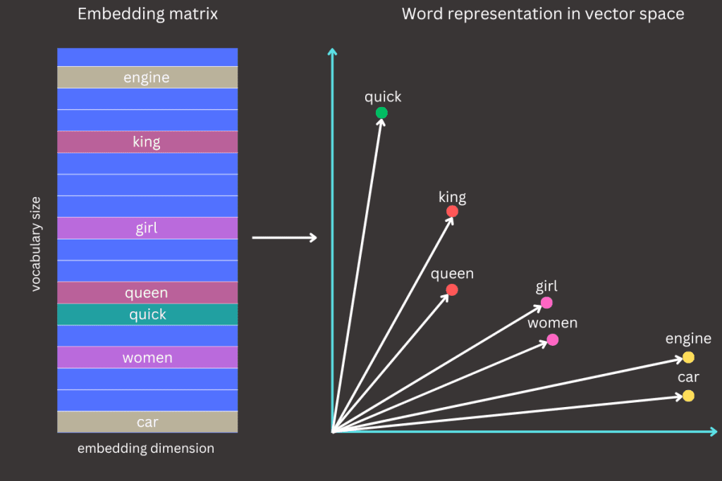
Each row in the embedding matrix corresponds to a unique word in the vocabulary, much like a specific address in an address book. The vector in that row represents the word’s location in a continuous, high-dimensional space.

For example, if the word quick is assigned an index of 101, the embedding matrix enables us to retrieve its corresponding vector representation, such as [0.2, -0.1, 0.3, … , 0.4]. The size of this vector is determined by the embedding dimension, which is specified before training begins.

These vectors can be visualized as coordinates in a high-dimensional space, where their positions capture semantic relationships. Words with similar meanings or contexts, such as king and queen, will have vector representations that are close to each other.

During the learning process, the embedding matrix is updated iteratively as the model trains on data. These updates capture the relationships between words, ensuring that words appearing in similar contexts have vector representations that reflect their semantic similarity. This dynamic adjustment allows the embedding matrix to encode meaningful patterns and relationships inherent in the language.

The embedding dimension is a predefined hyperparameter that determines the number of features or coordinates in each word vector. A higher embedding dimension allows for more expressive and nuanced representations of word meanings, capturing subtle semantic relationships. However, larger dimensions come with increased computational cost and may require more training data to prevent overfitting. On the other hand, smaller dimensions simplify computations but may lose finer semantic details.

Data preparation

Effective data preparation is a crucial step in training Word2Vec models, as the quality of the input data directly impacts the quality of the learned embeddings. This process involves transforming raw text into a format suitable for the model, including tokenization, vocabulary creation, and converting words into numerical representations. Additionally, techniques like subsampling are applied to reduce the dominance of frequent words and balance the dataset. Proper data preparation ensures that the model can focus on learning meaningful relationships between words, setting the foundation for successful training.

Building vocabulary

The vocabulary is a collection of all unique words in the training dataset, and its creation typically involves the following steps:

• Tokenization
  • Split the text into individual tokens (words or subwords).
  • This step often involves preprocessing, such as converting text to lowercase and removing punctuation or special characters
  • For example, the sentence The quick brown fox jumps over the lazy dog would be tokenized into the list: [the, quick, brown, fox, jumps, over, lazy, dog]
• Filtering Rare Words
  • Depending on the size of the dataset and computational constraints, rare words (those with frequencies below a threshold) may be excluded.
    • In the implementation used here, tokens that appear fewer than five times will be excluded from the vocabulary
  • This step helps reduce noise and memory usage
• Assigning Indexes
  • Each unique word in the vocabulary is assigned an integer index.
  • This index is used to map words to rows in the embedding matrix
• Special Tokens
  • Adding special tokens such as
    • <PAD> : for padding sequences to the same length
    • <UNK> : For unknown words that are not in the vocabulary
    • <SOS> / <EOS>: To mark the start or end of a sentence
  • In this blog and the accompanying implementation, we will exclusively use a special unknown token assigned to index 0

A summary of how to build a vocabulary is provided below, along with the corresponding code and an example of how to invoke the function.

dataset = "The quick brown fox jumps over the lazy dog"
vocabulary, token_couter = create_vocabulary(dataset)

# vocabulary
{
  '<unk>': 0,
  'The': 1,
  'quick': 2,
  'brown': 3,
  'fox': 4,
  'jumps': 5,
  'over': 6,
  'lazy': 7,
  'dog': 8
}

from collections import Counter


def create_vocabulary(text_dataset: str | list[str], top_k: int = 10_000) -> tuple[dict[str, int], Counter]:

    if type(text_dataset) == str:
        text_dataset_split = text_dataset.split(" ")
    else:
        text_dataset_split = text_dataset

    dataset_counter = Counter(text_dataset_split)

    vocab = {"<unk>": 0}
    vocab_idx = 1

    for word in dataset_counter.most_common(top_k - 1):
        w = word[0].strip()

        if dataset_counter[w] < 5:
            continue

        vocab[w] = vocab_idx
        vocab_idx += 1

    return vocab, dataset_counter

Data encoding

Each word or token in the dataset is replaced with its corresponding index from the vocabulary dictionary. This process transforms the raw text into numerical data that can be used by the model. For example, consider the simple sentence: The quick brown fox. Using the previously defined vocabulary, we can encode this text in two commonly used methods:

• One-Hot Encoding
  • In this approach, each word in the vocabulary is represented as a sparse vector of length V (the vocabulary size), where all elements are zero except for the position corresponding to the word’s index, which is set to one
  • For example, consider a vocabulary where the word quick is assigned the ID 2 and the vocabulary size is 10
    • Using one-hot encoding, quick would be represented as the vector: [0, 0, 1, 0, 0, 0, 0, 0, 0, 0]
    • When we deal with multiple words then each word is replaced with associated one-hot vector
      • For example, the dog would be represented as the matrix: [[0, 1, 0, 0, 0, 0, 0, 0, 0, 0], [0, 0, 0, 0, 0, 0, 0, 0, 0, 1]]
• Word Indices
  • Instead of creating a full one-hot vector, each word is simply assigned an integer index corresponding to its position in the vocabulary
    • For example, quick might be represented as 2 if it’s the second word
  • This method is both memory-efficient and computationally practical
    • During training, these indices are used to retrieve embeddings directly from the embedding matrix

Data encoding is essential because optimization algorithms cannot process strings directly; instead, they require numerical inputs. The two encoding methods discussed are among the most popular approaches for converting strings into numerical representations suitable for the learning process.

CBOW

The Continuous Bag of Words (CBOW) model forms the backbone of Word2Vec’s approach to learning word embeddings. Its task is simple yet powerful: given a set of context words (e.g., the, quick, fox), predict the target word (brown). This is achieved by leveraging a shallow neural network that transforms words into dense, numerical representations—embeddings.

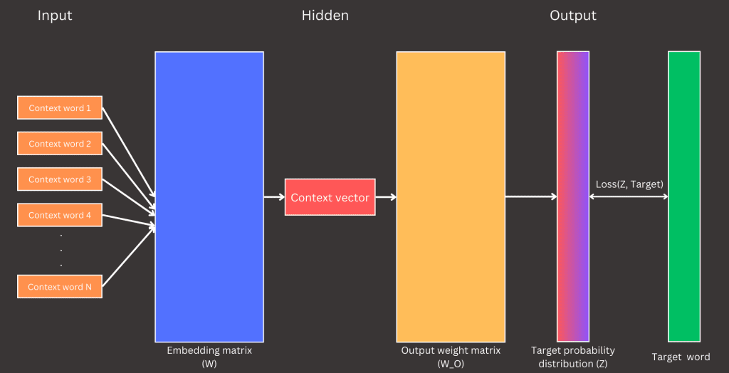
Imagine teaching a model to predict the missing word in the phrase: The quick __ fox. The CBOW model achieves this by averaging the embeddings of the context words (the, quick, fox) and passing this average through a softmax layer to predict the target word (brown). Let’s now break down each stage of the network to understand how data flows through it and how the computations are carried out.

The input layer of the CBOW model consists of the context words where the number of context words used during training is defined beforehand and is typically referred to as the window size (a term I often use). The window size specifies how many words are gathered around the target word to serve as input to the network. For instance, if the window size is 2, a total of 4 words (2 on each side of the target word) will be collected as context. Refer to Figure 4 for an illustration.

# example: The quick brown fox
# windows size = 2
context_words = ["the", "quick", "fox"]
target_word = ["brown"]

# convert words into indexes
context_words_ids = [1, 2, 4]
target_word_ids = [3]

The next step in this process (hidden layer) is to look up the embeddings for the context words in the embedding matrix and then average these vectors into a single vector suitable for the learning process. Context word indices are used to retrieve their corresponding word vectors from the embedding matrix, mapping each index to a specific vector in high-dimensional space. As a result, we obtain 2 x window size vectors, each with D dimensions, forming a tensor of shape (2 x window size, D). To proceed with the learning process, this tensor is averaged into a single vector of shape (D,).

# embedding dimension, D = 4
# windows size = 2

W = [
  [0.1,  0.2,  0.3,  0.4],    # <unk>
  [0.2,  0.1,  0.5,  0.9],    # the
  [0.2,  0.2,  0.3,  0.1],    # quick
  [0.05,  0.05,  0.1,  0.1],  # brown
  [0.1,  0.1,  0.6,  0.7],    # fox
  [0.75,  0.2,  0.3,  0.4],   # jumps
  [0.9,  0.9,  0.3,  0.3],    # over
  [0.02,  0.05,  0.01,  0.1], # lazy
  [0.1,  0.3,  0.4,  0.5]     # dog
]

context_words_ids = [1, 2, 4] # corresponse to words the, quick and fox
context_vectors = [
  [0.2,  0.1,  0.5,  0.9],    # the      <-> W[1]
  [0.2,  0.2,  0.3,  0.1],    # quick    <-> W[2]
  [0.1,  0.1,  0.6,  0.7],    # fox      <-> W[4]    
]

# operation like * and + are element-wise
averaged_context_vectors = 1/3 * (context_vectors[0] + context_vectors[1] + context_vectors[3]) = [0.1667, 0.1333, 0.4667, 0.5667]

The output layer is responsible for computing the probability distribution over all words in the vocabulary based on the input context. The resulting vector from this layer has a shape equal to the size of the vocabulary, representing the model’s predictions for each word.

How is this probability distribution computed? It starts with the dot product between the averaged context vector and the weights of the output layer. The averaged context vector has a shape of (D,), and the output weight matrix has a shape of (D, V), where D is the embedding dimension and V is the vocabulary size. The result is a vector of shape (V,), known as logits.

Logits are raw, unnormalized scores that indicate the model’s confidence in each word being the target. To transform these logits into a probability distribution, we apply the softmax function. The softmax operation converts the logits into probabilities by exponentiating each logit, normalizing them by dividing by the sum of the exponentials of all logits. The resulting probabilities are non-negative and sum to 1, making them suitable for predicting the target word.

W_O = [
    [0.1, 0.2, 0.3, 0.4, 0.5, 0.6, 0.7, 0.8, 0.9],
    [0.1, 0.3, 0.5, 0.7, 0.9, 1.1, 1.3, 1.5, 1.7],
    [0.2, 0.4, 0.6, 0.8, 1.0, 1.2, 1.4, 1.6, 1.8],
    [0.3, 0.5, 0.7, 0.9, 1.1, 1.3, 1.5, 1.7, 1.9]
]

# @ represents matrix multiplication
logits = averaged_context_vectors @ W_O = [0.4, 0.7534, 1.1067, 1.46, 1.8134, 2.1667, 2.52, 2.8734, 3.2267]

Z = softmax(logits) = [0.0184, 0.0262, 0.0373, 0.0531, 0.0756, 0.1077, 0.1532, 0.2181, 0.3104]

The final component of our neural network is the loss function, which defines the objective for the CBOW model and guides the learning process. In the CBOW model, the loss function measures the difference between the predicted probability distribution (computed from the softmax layer) and the true target word’s one-hot encoded representation. This comparison is typically made using the cross-entropy loss, a standard choice for classification tasks

The cross-entropy loss quantifies how well the predicted probabilities align with the actual target word. Mathematically, for a single target word, the loss is computed as:

Here, p_target represents the predicted probability of the correct target word. Let’s revisit our example to see this in action. The predicted probabilities from the softmax layer are:

Z = softmax(logits) = [0.0184, 0.0262, 0.0373, 0.0531, 0.0756, 0.1077, 0.1532, 0.2181, 0.3104]

In the vocabulary, the target word brown is at index 3. This means we take the value at index 3 from the predicted probabilities, which is 0.0531 . This value serves as p_target in the loss function and is used to compute the cross-entropy loss for this specific training sample.

Why do we convert the target word into a one-hot encoded format? In practical implementation, one-hot encoding simplifies the process of extracting the probability corresponding to the target word during loss computation. A one-hot encoded vector has a value of 1 at the index of the target word in the vocabulary and 0 at all other positions. When we multiply this one-hot encoded vector with the predicted probabilities ( Z ), all non-target probabilities are effectively eliminated (multiplied by 0), leaving only the probability of the correct target word. This makes the computation both efficient and straightforward.

Why do we convert the target word into a one-hot encoded format? In practical implementation, one-hot encoding simplifies the process of extracting the probability corresponding to the target word during loss computation. A one-hot encoded vector has a value of 1 at the index of the target word in the vocabulary and 0 at all other positions. When we multiply this one-hot encoded vector with the predicted probabilities ( Z ), all non-target probabilities are effectively eliminated (multiplied by 0), leaving only the probability of the correct target word. This makes the computation both efficient and straightforward.

Implementation

Let’s dive into the implementation details. We will use the JAX framework to build and train the CBOW model with data from the Wikipedia dataset, sourced via the Hugging Face Datasets library. Before exploring the specifics of the implementation, we’ll start by installing the required libraries, ensuring compatibility with Python 3.10.

pip install tqdm~=4.67
pip install datasets~=3.1
pip install nltk~=3.9
pip install plotly~=5.24
pip install scikit-learn~=1.5

# JAX CPU
pip install jax

# or GPU
# pip install "jax[cuda12]"

import re
import nltk

from tqdm.notebook import tqdm
from nltk.corpus import stopwords


nltk.download('punkt_tab')
nltk.download('stopwords')


def preprocess_text(text):
    text = text.lower()
    text = re.sub(r'[^\w\s]', '', text)
    tokens = nltk.word_tokenize(text)

    stop_words = set(stopwords.words('english'))
    tokens = [token for token in tokens if token not in stop_words]

    return tokens
    
    
TOP_K_ARTICLES = 50_000

en_wikipedia_dataset = load_dataset("wikipedia", "20220301.en")

train_text_tokens = []
for wiki_text in tqdm(en_wikipedia_dataset["train"].select(range(TOP_K_ARTICLES)), desc="Processing Wikipedia dataset", total=TOP_K_ARTICLES):
    train_text_tokens.extend(preprocess_text(wiki_text['text']))

Before diving into the JAX implementation, let’s first address how we process and prepare the data for input into the CBOW model. The goal is to take the dataset’s tokens and convert them into training samples, as illustrated in Figure 4. This involves iterating through the dataset tokens to construct context vectors (which serve as the input) and selecting target words (the output of the network). During this process, tokens are converted into indices based on a vocabulary built from the dataset. Additionally, we aim to implement batch learning to optimize the training process. This approach groups multiple training samples into batches, allowing for efficient computation and faster convergence during learning.

import numpy as np

from math import sqrt
from collections import Counter


def generate_training_text(
        tokens: list[str],
        vocabulary: dict[str, int],
        window_size: int = 2,
        stride: int = 1,
        batch_size: int | None = None,
        to_ids: bool = False
):
    len_tokens = len(tokens)
    range_len = len(range(window_size + 1, len_tokens - window_size - 1, stride))

    batch_context, batch_positives, batch_negatives = [], [], []
    for token_idx in range(window_size + 1, len_tokens - window_size - 1, stride):
        left_context = tokens[token_idx - window_size:token_idx]
        right_context = tokens[token_idx + 1:token_idx + window_size + 1]

        if to_ids:
            left_context_vector = [vocabulary.get(word, vocabulary["<unk>"]) for word in left_context]
            right_context_vector = [vocabulary.get(word, vocabulary["<unk>"]) for word in right_context]
            target_vector = vocabulary.get(tokens[token_idx], vocabulary["<unk>"])

            context_vector = left_context_vector + right_context_vector
        else:
            left_context_vector = left_context
            right_context_vector = right_context
            target_vector = tokens[token_idx]

            context_vector = left_context_vector + right_context_vector

        if target_vector == vocabulary["<unk>"]:
            continue


        if batch_size is None:
            yield context_vector, [target_vector, ]
        else:
            batch_context.append(context_vector)
            batch_positives.append(target_vector)

            if len(batch_positives) == batch_size:
                yield np.array(batch_context), np.array(batch_positives)
                batch_context, batch_positives = [], []

    if len(batch_positives) > 0 or len(batch_context) > 0:
        yield np.array(batch_context), np.array(batch_positives)

def remove_stopwords_and_common_words(tokens, additional_common_words=None):
    stop_words = set(stopwords.words('english'))

    if additional_common_words:
        stop_words.update(additional_common_words)

    filtered_tokens = [word.strip() for word in tokens if word.lower() not in stop_words and len(word) > 1]

    return filtered_tokens


def subsample_tokens(tokens: list[str], subsample_threshold: float = 1e-3) -> list[str]:
    total_words = len(tokens)
    word_counts = Counter(tokens)
    word_frequencies = {word: count / total_words for word, count in word_counts.items()}

    subsampling_probs = {
        word: (sqrt(freq / subsample_threshold) + 1) * (subsample_threshold / freq)
        if freq > subsample_threshold else 1.0
        for word, freq in word_frequencies.items()
    }

    sub_sampled_tokens = []
    for word in tqdm(tokens, desc="Subsampling tokens"):
        random_value = np.random.rand()
        if random_value < subsampling_probs[word]:
            sub_sampled_tokens.append(word)

    return sub_sampled_tokens


TOP_K = 30_000
STRIDE = 1
WINDOWS_SIZE = 10

# create vocabulary from the dataset
train_dataset = remove_stopwords_and_common_words(train_text_tokens)
train_dataset = subsample_tokens(train_dataset, 1e-5)
vocabulary, _ = create_vocabulary(train_dataset, top_k=TOP_K)

train_dataset = [word for word in train_dataset if vocabulary.get(word, 0)]
train_token_counter = Counter(train_dataset)
len_train_dataset_tokens = len(train_dataset)


for context_words, target_words in generate_training_text(train, vocabulary, window_size=WINDOWS_SIZE, stride=STRIDE, batch_size=4, to_ids=False):
    print(f"Context words: {context_words}")
    print(f"Target words: {target_words}")
    
    break


# Output:    
Context words: [['sceptical' 'authority' 'rejects' 'involuntary' 'coercive' 'hierarchy'
  'anarchism' 'calls' 'abolition' 'holds' 'undesirable' 'harmful'
  'leftwing' 'placed' 'farthest' 'spectrum' 'libertarian' 'marxism'
  'libertarian' 'wing']
 ['authority' 'rejects' 'involuntary' 'coercive' 'hierarchy' 'anarchism'
  'calls' 'abolition' 'holds' 'unnecessary' 'harmful' 'leftwing' 'placed'
  'farthest' 'spectrum' 'libertarian' 'marxism' 'libertarian' 'wing'
  'libertarian']
 ['rejects' 'involuntary' 'coercive' 'hierarchy' 'anarchism' 'calls'
  'abolition' 'holds' 'unnecessary' 'undesirable' 'leftwing' 'placed'
  'farthest' 'spectrum' 'libertarian' 'marxism' 'libertarian' 'wing'
  'libertarian' 'socialism']
 ['involuntary' 'coercive' 'hierarchy' 'anarchism' 'calls' 'abolition'
  'holds' 'unnecessary' 'undesirable' 'harmful' 'placed' 'farthest'
  'spectrum' 'libertarian' 'marxism' 'libertarian' 'wing' 'libertarian'
  'socialism' 'socialist']]
Target words: ['unnecessary' 'undesirable' 'harmful' 'leftwing']



for context_words, target_words in generate_training_text(train, vocabulary, window_size=WINDOWS_SIZE, stride=STRIDE, batch_size=4, to_ids=True):
    print(f"Context words: {context_words}")
    print(f"Target words: {target_words}")
    
    break
    
# Output (ids):
Context words: [[26281   793 10216 16770 24137  5968  9742  2348  6752  2047 15105  7996
   8543   841 19884  3197  9019 13834  9019  2335]
 [  793 10216 16770 24137  5968  9742  2348  6752  2047  9622  7996  8543
    841 19884  3197  9019 13834  9019  2335  9019]
 [10216 16770 24137  5968  9742  2348  6752  2047  9622 15105  8543   841
  19884  3197  9019 13834  9019  2335  9019  5486]
 [16770 24137  5968  9742  2348  6752  2047  9622 15105  7996   841 19884
   3197  9019 13834  9019  2335  9019  5486  2338]]
Target words: [ 9622 15105  7996  8543]



BATCH_SIZE = 2048

print("Generating dataset")
full_dataset = list(generate_training_text(train, vocabulary, window_size=WINDOWS_SIZE, stride=STRIDE, batch_size=BATCH_SIZE, to_ids=True))

The function generates batches of context words and corresponding target words, with the batch size specified by the batch_size parameter. The window_size parameter determines the number of context words to include around the target word, as described earlier. Additionally, the function includes an option (to_ids parameter) to specify whether the output should return words as strings or as indices mapped from the vocabulary. One parameter used during dataset preparation is set during vocabulary creation. To limit the number of words included in the vocabulary, we specify the desired number of words (TOP_K) in the create_vocabulary() function. This parameter ensures that only the most frequent words, based on their occurrence count, are retained in the vocabulary.

Training

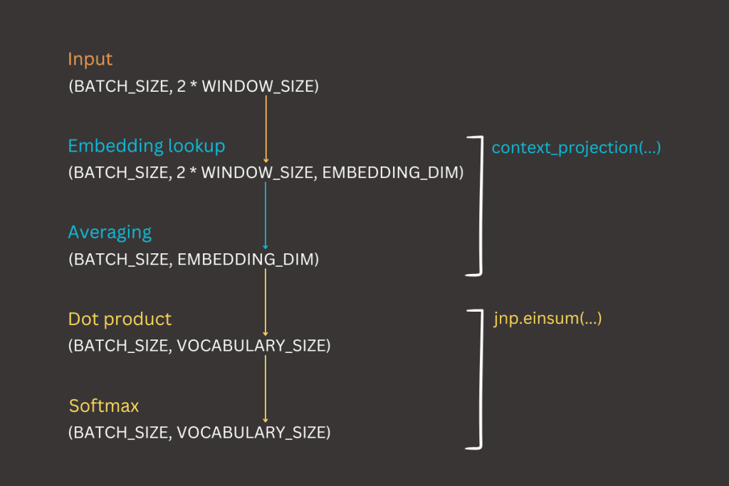
What is required to implement CBOW in JAX? With the data now prepared for the learning process, the next steps are straightforward. As shown in Figure 7, the CBOW model relies on two sets of weights in its hidden layer. The first is the embedding matrix (W), a tensor with a shape of (vocabulary size, embedding dimension), which maps words to their vector representations. The second is the output weight matrix, a tensor with a shape of (embedding dimension, vocabulary size), which converts the averaged context vector into logits over the vocabulary. Remember, the embedding dimension is a parameter that must be defined before the learning process begins. In our example, we will use an embedding dimension of 300, which is a common choice. Other popular options include 50, 100, and 200, depending on the complexity of the task and the available computational resources.

EMBEDDING_DIM = 300

embedding_init = jax.nn.initializers.glorot_uniform()

cbow_params = {
    "embedding": embedding_init(jax.random.PRNGKey(69), (len(vocabulary), EMBEDDING_DIM)),
    "output": embedding_init(jax.random.PRNGKey(69), (EMBEDDING_DIM, len(vocabulary)))
}

Let’s define the feedforward process, which involves the sequence of computations that transform the input into the output in a neural network. The detailed forward process has already been explained in the CBOW section. Here, we will focus on explaining how tensor shapes evolve throughout the forward process.

• Input context vectors
  • Shape: (BATCH_SIZE, 2 * WINDOW_SIZE)
• Embedding Retrieval and Averaging
  • Shape: (BATCH_SIZE, EMBEDDING_DIMENSION)
  • The context word indices are used to retrieve their corresponding embeddings from the embedding matrix (W)
  • These embeddings are then averaged across the context dimension to create a single context vector for each sample in the batch
• Output probabilities distribution
  • Shape: (BATCH_SIZE, VOCABULARY_SIZE)
  • The averaged context vector is multiplied by the output weight matrix (W_O) using a dot product, resulting in logits
  • These logits are then converted into a probability distribution over the vocabulary

@jax.jit
def context_projection(params, context_samples):
    context_vector_state = params["embedding"][context_samples]

    return jnp.mean(context_vector_state, axis=1)  # (BATCH, EMBEDDING_DIMENSION)


@jax.jit
def forward(params, context_vector):
    context_projection_result = context_projection(params, context_vector) # (BATCH_SIZE, EMBEDDING_DIMENSION)
    context_projection_dot_result = jnp.einsum("be,ev->bv", context_projection_result, params["output"]) # (BATCH_SIZE, VOCAB_SIZE)

    return context_projection_dot_result # (BATCH_SIZE, VOCAB_SIZE)
    
    
    
for context_words, target_words in generate_training_text(train, vocabulary, window_size=WINDOWS_SIZE, stride=STRIDE, batch_size=4, to_ids=True):
    print(f"Context words: {context_words}")
    print(f"Target words: {target_words}")
    break


forward(cbow_params, context_words)
forward(cbow_params, context_words).shape

# Output
Context words: [[ 674 9644 4454 5451 2647 2018 9885 8076 8680  839]
 [9644 4454 5451 2647 6465 9885 8076 8680  839 2578]
 [4454 5451 2647 6465 2018 8076 8680  839 2578 7284]
 [5451 2647 6465 2018 9885 8680  839 2578 7284 7284]]
Target words: [6465 2018 9885 8076]

Array([[ 7.8612240e-04,  1.6868199e-04,  1.0352904e-03, ...,
         1.3179374e-03, -4.5935644e-04, -6.4104376e-04],
       [ 9.2905987e-04, -4.2303978e-04,  1.2492843e-03, ...,
         1.5665784e-03,  1.3830396e-04,  5.9611135e-04],
       [ 6.9052743e-04,  7.3607994e-04,  1.8318576e-03, ...,
         1.8510298e-03, -2.8697564e-04, -6.5784337e-04],
       [ 3.0725828e-04,  3.5895078e-04,  2.5489661e-03, ...,
         2.7622725e-03, -6.5552449e-05, -2.7063324e-03]], dtype=float32)
         
(4, 10000)         

The missing component in the implementation is the loss function. One of the advantages of JAX is that, once we implement a JAX-compatible loss computation, obtaining gradients for parameter updates becomes an implicit process. This approach has been detailed earlier in this blog post, where gradient updates were demonstrated using linear regression as an example.

@jax.jit
def loss_fn(params, context_vector, target):
    logits = forward(params, context_vector)  # (BATCH_SIZE, VOCAB_SIZE)

    target_ohe = jax.nn.one_hot(target, len(vocabulary)) # (BATCH_SIZE, VOCAB_SIZE)
    loss_result = optax.losses.softmax_cross_entropy(logits, target_ohe).mean() # (BATCH_SIZE,)

    return loss_result

This loss function follows the approach described in the previous section, where the one-hot encoded target vector is combined with the computed logits to calculate the loss using the Optax library’s softmax_cross_entropy function. One detail worth mentioning is that the conversion of the target word to a one-hot encoded format occurs directly within the loss function implementation using a JAX function. While there is no specific reason for performing the conversion here, it could alternatively be done during the dataset preparation stage. In such a case, the conversion step could be omitted from the loss function entirely.

def shuffle_dataset(dataset):
    np.random.shuffle(dataset)

    for (context_vector, target_vector) in dataset:
        yield context_vector, target_vector
        
        
LR = 1e-3
EPOCHS = 25


optimizer = optax.adam(learning_rate=LR)
opt_state = optimizer.init(cbow_params)


training_loss = []
with tqdm() as training_progress:
    for epoch_id in range(EPOCHS):
        training_progress.set_description(f"Training: Epoch {epoch_id + 1}/{EPOCHS}")
        training_progress.reset(total=len(full_dataset))

        training_epoch_loss = []
        for (context_vector, target_vector) in shuffle_dataset(full_dataset):
            value_of_loss, grads = jax.value_and_grad(loss_fn)(cbow_params, context_vector, target_vector)
            updates, opt_state = optimizer.update(grads, opt_state)
            cbow_params = optax.apply_updates(cbow_params, updates)

            training_epoch_loss.append(value_of_loss)

            training_progress.set_postfix({"loss": value_of_loss})
            training_progress.update(1)

        training_loss.append(np.mean(training_epoch_loss))

The training loop, once all components are defined, is a straightforward process. In this implementation, we use the Optax optimizer to update the trainable parameters: the embedding matrix (W) and the output weight matrix (W_O). The usage of Optax has been briefly described earlier in this blog post. Before starting the training process, two key hyperparameters must be defined: the learning rate and the number of epochs. For the purpose of this blog, these are set to 1e-3 (0.001) and 25 epochs, respectively, which should suffice to achieve reasonable results on the dataset.

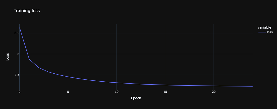
After completing the training process, we can explore the trained embeddings to evaluate the results. However, before analyzing the embedding matrix, it is important to first examine the training loss. We expect the training loss to show a decreasing trend over time (across epochs), indicating that the model is learning effectively. While the exact loss value may vary depending on the experiment and parameters used, the general trend is a key indicator of progress. For the experiment conducted in this blog, the loss trend is illustrated in Figure 12.

The following hyperparameters were used during training for this blog post:

• TOP_K_ARTICLES
  • Defines the number of articles loaded from Wikipedia using the Hugging Face datasets library
  • Value: 50 000
• TOP_K
  • Specifies the number of tokens retained in the vocabulary after filtering
  • Value: 30 000
• WINDOW_SIZE
  • Determines the number of context words to include on each side of the target word
  • Value: 10
• EMBEDDING_DIM
  • Sets the dimensionality of the embedding vectors in the embedding matrix
  • Value: 300
• LR (learning rate)
  • Controls the step size for weight updates during optimization
  • Value: 1e-3
• EPOCHS
  • Specifies the number of complete passes through the training data
  • Value: 25 epochs
• BATCH_SIZE
  • Defines the number of samples included in each training batch
  • Value: 2048

Extracting Embeddings

At the beginning of this blog, we discussed how Word2Vec models learn relationships between words. Now, it’s time to explore these relationships in action. To explore the properties of the embedding matrix, we will implement two key functions: find_most_similar_words and resolve_analogy. These functions will allow us to retrieve similar words for a given word and solve word analogies, respectively.

• find_most_similar_words
  • Identifies the top N most similar words to a given word based on their embeddings
  • Arguments
    • word: The input word for which we want to find similar words
    • vocabulary: A dictionary mapping words to their indices
    • embeddings: The embedding matrix representing word vectors
    • top_n: The number of similar words to retrieve (default is 5)
  • Returns a list of the top N most similar words along with their similarity scores
• resolve_analogy
  • Resolves analogies of the form: Word A is to Word B as Word C is to Word D
  • Arguments
    • word_a, word_b, word_c: Words forming the analogy input
    • vocabulary: A dictionary mapping words to their indices
    • embeddings: The embedding matrix representing word vectors
    • top_n: The number of potential answers to retrieve (default is 1)
  • Returns the top N most similar words that complete the analogy, along with their similarity scores

from sklearn.metrics.pairwise import cosine_similarity


def find_most_similar_words(word, vocabulary, embeddings, top_n=5):

    if word not in vocabulary:
        raise ValueError(f"Word '{word}' not found in the vocabulary.")

    word_idx = vocabulary[word]
    target_embedding = embeddings[word_idx].reshape(1, -1)  # Shape: (1, EMBEDDING_DIM)

    similarities = cosine_similarity(target_embedding, embeddings)[0]  # Shape: (VOCAB_SIZE,)

    similar_indices = similarities.argsort()[::-1]
    similar_indices = [idx for idx in similar_indices if idx != word_idx]

    reverse_vocab = {idx: w for w, idx in vocabulary.items()}
    similar_words = [(reverse_vocab[idx], float(similarities[idx])) for idx in similar_indices[:top_n]]

    return similar_words
    
    
find_most_similar_words("computer", vocabulary, cbow_params["embedding"], top_n=10)    
[('computers', 0.6549213528633118),
 ('computing', 0.5817990303039551),
 ('software', 0.5484875440597534),
 ('programmers', 0.46077266335487366),
 ('machines', 0.4445808529853821),
 ('hardware', 0.43988996744155884),
 ('machine', 0.42370492219924927),
 ('graphics', 0.3857647478580475),
 ('electronics', 0.38181865215301514),
 ('electronic', 0.3812060058116913)]
 
 
find_most_similar_words("news", vocabulary, cbow_params["embedding"], top_n=10)
[('newspapers', 0.5128046274185181),
 ('newspaper', 0.4866177439689636),
 ('cnn', 0.45792531967163086),
 ('coverage', 0.44172507524490356),
 ('journalists', 0.4307379126548767),
 ('journalism', 0.424543559551239),
 ('correspondent', 0.4166100025177002),
 ('weekly', 0.41641008853912354),
 ('outlets', 0.3953128457069397),
 ('broadcasts', 0.39508721232414246)]
 
 
find_most_similar_words("war", vocabulary, cbow_params["embedding"], top_n=10)
[('military', 0.4897465705871582),
 ('allies', 0.4876498579978943),
 ('army', 0.473164439201355),
 ('wars', 0.4709010720252991),
 ('allied', 0.44286447763442993),
 ('battles', 0.4426190257072449),
 ('wartime', 0.4399275481700897),
 ('battle', 0.4290524125099182),
 ('ii', 0.4244605004787445),
 ('soldiers', 0.41415101289749146)]
 
find_most_similar_words("paris", vocabulary, cbow_params["embedding"], top_n=10)
[('france', 0.5458036661148071),
 ('french', 0.5205941200256348),
 ('parisian', 0.5124962329864502),
 ('le', 0.44794511795043945),
 ('sorbonne', 0.44427770376205444),
 ('henri', 0.436335027217865),
 ('francs', 0.43554043769836426),
 ('rue', 0.431929349899292),
 ('palais', 0.42690974473953247),
 ('montmartre', 0.4266318082809448)]

From the results, we can see that the retrieved words for each given input make logical sense based on the dataset. For example, words like computers, software, and hardware are closely related to computer, while newspapers, journalists, and broadcasts are retrieved for news. Similarly, military, army, and soldiers are associated with war, and france, french, and parisian are relevant to paris. This demonstrates that the model successfully captures semantic relationships and groups words based on their context and meaning in the dataset.

from sklearn.metrics.pairwise import cosine_similarity


def resolve_analogy(word_a, word_b, word_c, vocabulary, embeddings, top_n=1):

    for word in [word_a, word_b, word_c]:
        if word not in vocabulary:
            raise ValueError(f"Word '{word}' not found in the vocabulary.")

    idx_a, idx_b, idx_c = vocabulary[word_a], vocabulary[word_b], vocabulary[word_c]
    embedding_a, embedding_b, embedding_c = embeddings[idx_a], embeddings[idx_b], embeddings[idx_c]

    analogy_vector = embedding_b - embedding_a + embedding_c

    similarities = cosine_similarity(analogy_vector.reshape(1, -1), embeddings)[0]  # Shape: (VOCAB_SIZE,)

    sorted_indices = similarities.argsort()[::-1]
    excluded_indices = {idx_a, idx_b, idx_c}
    sorted_indices = [idx for idx in sorted_indices if idx not in excluded_indices]

    reverse_vocab = {idx: word for word, idx in vocabulary.items()}
    similar_words = [(reverse_vocab[idx], float(similarities[idx])) for idx in sorted_indices[:top_n]]

    return similar_words
  

resolve_analogy(
    "king", "queen", "man",
    vocabulary, cbow_params["embedding"], top_n=5
)
[('woman', 0.34776929020881653),
 ('mary', 0.34084659814834595),
 ('love', 0.3265678286552429),
 ('lucy', 0.3248634338378906),
 ('never', 0.2979058623313904)]


resolve_analogy(
    "paris", "france", "berlin",
    vocabulary, cbow_params["embedding"], top_n=5
)
[('germany', 0.4728545546531677),
 ('german', 0.3924347460269928),
 ('berlins', 0.3764692544937134),
 ('germanys', 0.3745086193084717),
 ('gdr', 0.36564379930496216)]
 
 
 resolve_analogy(
    "euro", "europe", "dollar",
    vocabulary, cbow_params["embedding"], top_n=5
)
[('america', 0.30482083559036255),
 ('china', 0.28317785263061523),
 ('pacific', 0.2670055031776428),
 ('imports', 0.25992637872695923),
 ('americas', 0.2519795894622803)]

An analogy in word embeddings involves discovering relationships between words based on the mathematical operations performed on their vector representations. The classic example is: king is to queen as man is to ?.

In terms of word vectors, this analogy can be represented as:

By rearranging this, we compute the vector for the unknown word as:

which is exactly what is implemented in the resolve_analogy function.

Summary

In this blog post, we explored into the CBOW (Continuous Bag of Words) model, a foundational technique in Word2Vec, and implemented it step by step using JAX. Starting with data preparation, we tokenized text, created a vocabulary, and generated training samples. We then built the CBOW model, explained its architecture, and demonstrated how embeddings are learned by predicting target words from their context.

The JAX implementation highlighted how its simplicity and efficiency make it easier to transition from an idea to a fully functional training process. By leveraging JAX’s capabilities for automatic differentiation and just-in-time compilation, we streamlined the development of the CBOW model, focusing on both performance and clarity. Finally, we evaluated the embeddings by retrieving similar words and solving analogies, showcasing the meaningful relationships captured by the model.

The complete code is available as a notebook here.
The weights used in this blog post are stored at this location. They are saved in the same format as used during the training process (cbow_params).