Clustering with Union-Find: Single-Linkage Implementation

In this post, we’ll explore how the union-find data structure functions and its importance in machine learning applications. We’ll specifically focus on its role in clustering algorithms, demonstrating how it helps manage dynamic cluster formation and identify connected components efficiently. By implementing hierarchical clustering, you’ll see firsthand how this structure enhances the performance of algorithms, especially when handling large datasets.

Introduction

How do we efficiently determine if two elements belong to the same group? If they don’t, how can we quickly merge two groups together while maintaining the ability to check this in the future? These are fundamental questions that arise in various computational problems, from dynamic clustering and network connectivity to image segmentation and more.

Formally, consider a list of pairs of numbers, where each number represents an object. For each pair (p, q), we say “p is connected to q”, this connection follows a few basic rules: every object is connected to itself (p is connected to p), if p is connected to q, then q is also connected to p, and if p is connected to q and q is connected to r, then p is connected to r. This type of relationship is known as an equivalence relation, and it divides the objects into equivalence classes. Two objects belong to the same class if and only if they are connected.

The union-find data structure answers these questions efficiently. By managing disjoint sets and providing operations to merge sets and check relationships between elements, union-find allows us to solve problems involving connected components and set membership with near constant time complexity. This structure plays a critical role in a range of algorithms where tracking relationships between elements over time is essential, such as in clustering, graph analysis, and beyond.

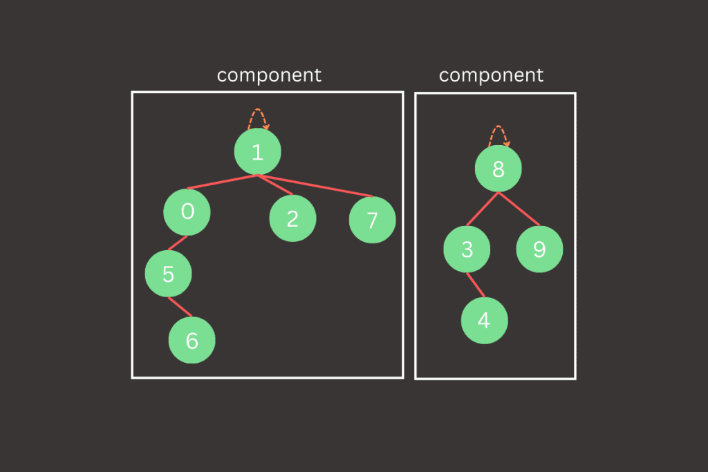
In the example shown in Figure 3, the nodes are labeled from 0 to 9, and we are connecting them based on the pairs of numbers given in the sequence. Each pair represents an operation where two nodes are linked, forming a new connection between them. To better understand what this sequence might represent in a real-world scenario, imagine the nodes are cities, and each pair in the sequence indicates that a direct road is being built between two cities. As more roads are built, the cities gradually become part of a larger, interconnected road network. Just like in this example, if a city is already reachable through existing roads, no new road needs to be built between them, which optimizes the process.

Each pair, such as (4, 3), represents an operation where two nodes—here, nodes 4 and 3—are connected, creating a new link between them. This connection can be visualized as drawing a line between the two nodes, making them part of the same group, or component.

As we move through the sequence, we continue connecting more pairs of nodes. For instance, after connecting (4, 3), we connect (3, 8), which links node 8 to the existing group formed by nodes 3 and 4. Similarly, other pairs like (6, 5) and (9, 4) further build out different groups.

At certain points, a pair may involve nodes that are already connected indirectly through other nodes. For example, when we reach the pair (8, 9), node 8 is already connected to node 9 through the path 8 → 3 → 4 → 9. In this case, the pair is not printed or processed, since no new connection is needed. This helps avoid redundant operations and demonstrates the efficiency of the union-find structure.

By the end of this process, all nodes have been grouped into larger connected components. In this case, we end up with two fully connected components, where each node is either directly or indirectly connected to every other node in its component.

In the following sections, we will dive deeper into the union-find data structure, exploring its operations and significance. We’ll also walk through how to implement it effectively for clustering tasks, illustrating its practical applications in efficiently managing dynamic cluster formation.

Union-Find: Implementation Overview

With the union-find structure, our goal is to efficiently answer the question: Are two given objects (or sites) in a network connected? This connection can represent any type of relationship depending on the problem context. Additionally, we aim to ensure that forming new connections is as optimal as possible within this framework, minimizing redundant operations while maintaining efficiency. In this blog, we will stick to network terminology and refer to the objects as nodes, the pairs as connections and the equivalence classes as connected components (or just components).

With this premise in mind, we can now define a class that encapsulates the union-find structure;

class UnionFind:    
    def find(self, p)
    def union(self, p, q)
    def connected(self, p, q)

The find() method in this class will take a node identifier as an argument and return the component identifier it belongs to. The union() method will take two nodes and establish a connection between them. Finally, the connected() method will take two nodes and return true if they are part of the same component, and false otherwise and method count() which return number of components. For simplicity, we’ll assume that node IDs are represented by integers, and if we have N nodes in the network, they will be numbered from 0 to N-1. In practice, node IDs could be more complex types, and with minor adjustments to the code, these could be supported. However, for the purpose of this blog post, this level of complexity isn’t necessary, as most real-world applications can be effectively handled with simple integer-based enumeration.

Python

class UnionFind:

    def __init__(self, size: int):
        self.nodes = [i for i in range(size)]
        self.count = size
        
    def find(self, p):
        pass

    def union(self, p, q):
        pass
    
    def connected(self, p, q):
        pass
                
    
        

Abstract union-find structure

With this problem setup, we can begin implementing the structure, and it makes sense to use an array of integers called nodes[], which will represent the components in the network. Each component will be identified by one of its nodes, meaning we use a node’s ID as the component identifier. Initially, since we have N nodes, each node is its own component. Therefore, we initialize nodes[i] to i for all nodes from 0 to N-1, representing that each node is its own component at the start. For each node i, we store the necessary information that the find() method will need to determine which component the node belongs to. In this case, the nodes[] array keeps track of the component identifier for each node, so the find() method can quickly lookup and return the component to which a node belongs.

Quick find

The first implementation we’ll present focuses on a quick and efficient way to determine whether two nodes are connected and belong to the same component. This approach maintains the rule that p and q are connected if, and only if, nodes[p] is equal to nodes[q]. In simple terms, all nodes in the same component will share the same value in the nodes[] array. Refer to Figure 4 for a visual representation.

Python

class UnionFind:

    def __init__(self, size: int):
        self.nodes = [i for i in range(size)]
        self.count = size

    def find(self, p):
        return self.nodes[p]

    def union(self, p, q):
        pass

    def connected(self, p, q):
        return self.nodes[p] == self.nodes[q]

Partial implementation of quick find union find structure

After understanding how the connected() method works, implementing the union() method becomes straightforward. The union() method updates connections by ensuring that all nodes in the same component share the same identifier. When merging or connecting two nodes, we need to ensure that not only the nodes passed as arguments get the same identifier, but also all other nodes in their respective components.

Python

class UnionFind:

    def __init__(self, size: int):
        self.nodes = [i for i in range(size)]
        self.count = size

    def find(self, p):
        return self.nodes[p]

    def union(self, p, q):
        p_id = self.find(p)
        q_id = self.find(q)

        if p_id != q_id:
            for i in range(len(self.nodes)):
            
                if self.nodes[i] == p_id:
                    self.nodes[i] = q_id
                    
            self.count -= 1

    def connected(self, p, q):
        return self.nodes[p] == self.nodes[q]

Quick find implementation

With the union-find structure now fully implemented, we can analyze the performance of the operations, focusing on the number of accesses to the nodes[] array. The find() method, and by extension the connected() method, are highly efficient, requiring only a single access to the nodes[] array to retrieve the component identifier of a node. However, the union() method is less efficient, as it must scan the entire nodes[] array to update all nodes belonging to the same component. This makes the current implementation inefficient for large datasets, since the union() operation, in the worst case, can involve multiple accesses to the array, resulting in a quadratic-time process.

Quick union

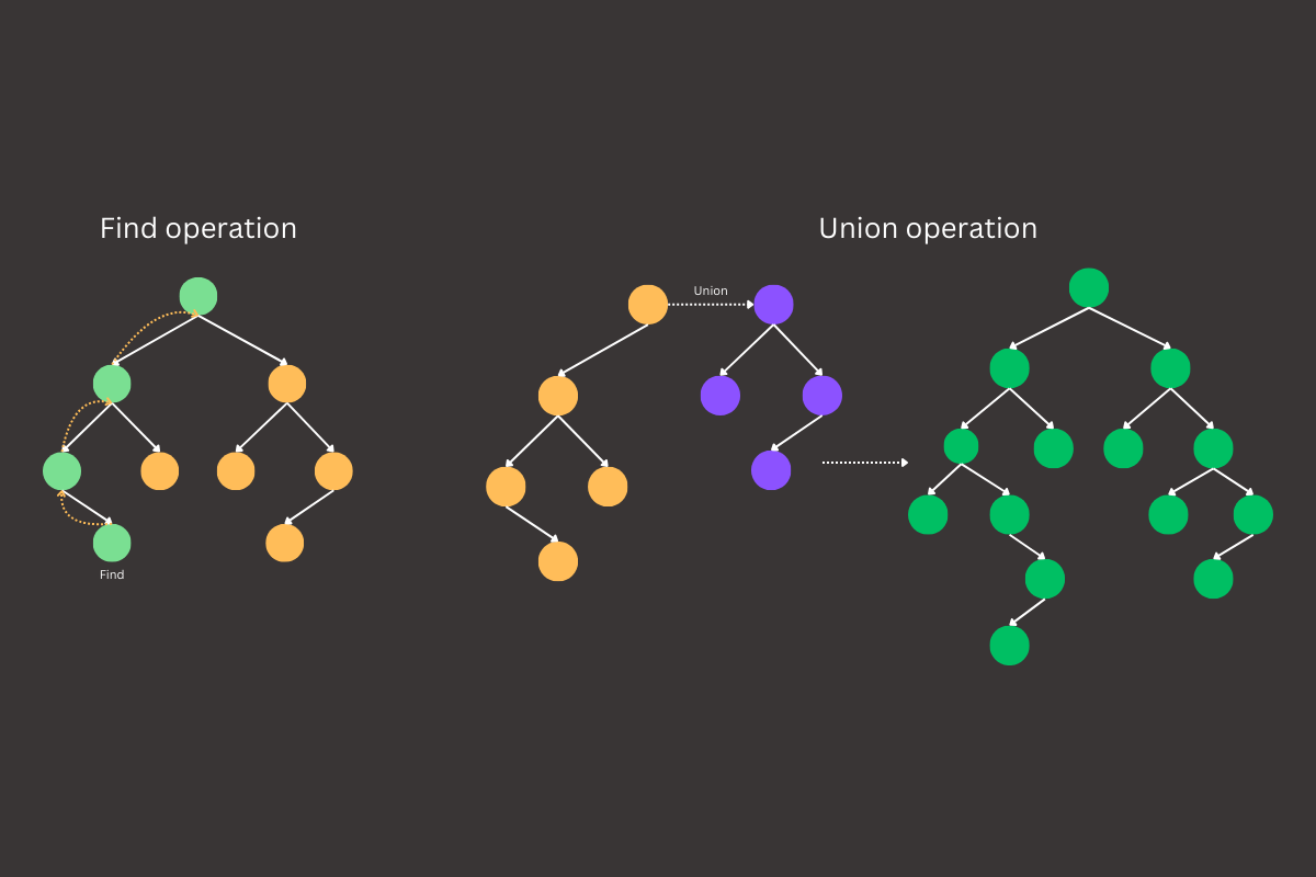
Now, we’ll shift our focus to optimizing the union() method while still using the nodes[] data structure. However, the way we interpret the values stored in the nodes[] array will change and become a bit more involved. Previously, each node directly stored its component identifier, but now each entry in nodes[] will point to another node within the same component. This link can either point to a different node or, in the case of the root node, point to itself. If you take a closer look, you’ll notice that we’ve essentially created a forest of trees within the union-find data structure, where each node points to its parent, and the roots serve as the representatives of their respective components.

The find() method will work by starting at a given node (let’s say p) and following the link from p to another node. This process continues from node to node, following links, until it reaches the root—a node that points to itself. This root acts as the representative of the entire component. For two nodes to be in the same component, they must share the same root. In other words, the find() method will trace the path from each node to its root, and if both nodes have the same root, they are part of the same component. This approach adds some complexity compared to the previous version, but it lays the groundwork for a more efficient union() method by reducing the number of updates needed during each union operation.

The union() method will need to maintain the process we just described. Fortunately, this is straightforward to implement. Let’s say we want to connect two nodes, p and q. To do this, we first need to find the root node for each of them, which involves following the links from p and q to their respective root nodes.

Python

class UnionFind:

    def __init__(self, size: int):
        self.nodes = [i for i in range(size)]
        self.count = size

    def find(self, p: int):
        while p != self.nodes[p]:
            p = self.nodes[p]

        return p

    def connected(self, p: int, q: int):
        return self.find(p) == self.find(q)

    def union(self, p: int, q: int):
        p_root = self.find(p)
        q_root = self.find(q)

        if p_root != q_root:
            self.nodes[p_root] = q_root
            self.count -= 1

Quick union implementation

If these two roots are different, it means that p and q belong to different components, and we can merge them by linking one root to the other. Essentially, we rename one of the components by connecting the root of one component to the root of the other. This action effectively merges the two components, ensuring that both p and q (along with all the nodes in their respective components) now share the same root, and are thus part of the same unified component.

Using a similar analysis as with the quick-find implementation, we can see that the quick-union implementation has a much faster union() operation because it doesn’t need to scan the entire array for each input. However, the question remains: how much faster is the overall process? In the best-case scenario, the find() operation only requires one array access to locate the node. But in the worst case, it can take up to O(N) array accesses, as illustrated in Figure 9.

This happens because, in the worst-case scenario, the find() operation might have to traverse through every node in a deep linear tree to reach the root. If we perform N union() operations that each result in this worst-case linear structure, then every subsequent find() operation will need O(N) accesses to locate the root. Since there could be multiple such find() operations, the overall complexity can accumulate to O(N²), making the entire process quadratic in the worst case.

Weighted quick union

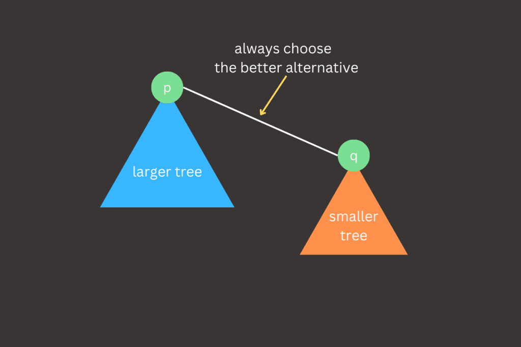
There is a simple modification we can make to our implementation to prevent bad cases like linear tree growth. Instead of arbitrarily connecting one tree to another in the union() method, we can introduce an additional array, called size[], to keep track of the size of each tree. This allows us to always connect the smaller tree to the larger one. By doing this, we ensure that the overall tree structure remains balanced, avoiding the formation of deep, inefficient trees.

Python

class UnionFind:

    def __init__(self, size: int):
        self.nodes = [i for i in range(size)]
        self.sizes = [1 for i in range(size)]
        self.count = size

    def find(self, p):
        while p != self.nodes[p]:
            p = self.nodes[p]

        return p

    def connected(self, p, q):
        return self.find(p) == self.find(q)

    def union(self, p, q):
        p_root = self.find(p)
        q_root = self.find(q)

        if p_root != q_root:

            if self.sizes[p_root] < self.sizes[q_root]:
                self.nodes[p_root] = q_root
                self.sizes[q_root] += self.sizes[p_root]
            else:
                self.nodes[q_root] = p_root
                self.sizes[p_root] += self.sizes[q_root]

            self.count -= 1

Weighted quick union implementation

The worst-case scenario for the weighted quick union implementation occurs when the trees being merged by union() are always equal in size, specifically when their sizes are powers of 2. Although these tree structures may seem complex, they follow a simple property: the height of a tree with 2ⁿ nodes is n. When we merge two trees, each with 2ⁿ nodes, the resulting tree will have 2ⁿ⁺¹ nodes, and its height increases to n+1. This pattern provides a clear proof that the weighted quick union implementation ensures O(log N) performance, as the height of the trees grows logarithmically with the number of nodes.

The weighted quick union implementation is efficient enough to handle larger datasets and is well-suited for real-world applications. However, there are additional optimizations that can make this structure even faster, such as path compression. Path compression improves the find() operation by moving the nodes it inspects directly to the root, further speeding up future queries.

Path compression is a simple but powerful optimization that can be easily added to the current implementation. It involves adding an additional loop in the find() method to update each node encountered along the path, making it point directly to the root. This flattens the tree, improving efficiency for future operations. Beyond path compression, there are other one-pass find() optimizations like path splitting and path halving, which also update the parent pointers along the path to the root. Path splitting, for example, replaces each parent pointer with a pointer to the node’s grandparent, further reducing the path length and enhancing efficiency while maintaining the same worst-case complexity.

Python

class UnionFind:

    def __init__(self, size: int):
        self.nodes = [i for i in range(size)]
        self.sizes = [1 for i in range(size)]
        self.count = size

    def find(self, p):
        root = p
        while root != self.nodes[root]:
            root = self.nodes[root]

        while p != self.nodes[p]:
            next_node = self.nodes[p]
            self.nodes[p] = root
            p = next_node

        return root

    def connected(self, p, q):
        return self.find(p) == self.find(q)

    def union(self, p, q):
        p_root = self.find(p)
        q_root = self.find(q)

        if p_root != q_root:

            if self.sizes[p_root] < self.sizes[q_root]:
                self.nodes[p_root] = q_root
                self.sizes[q_root] += self.sizes[p_root]
            else:
                self.nodes[q_root] = p_root
                self.sizes[p_root] += self.sizes[q_root]

            self.count -= 1

Path compression implementation

The implementations of path halving and path splitting are fairly straightforward, requiring only a minor modification to the find() method with the addition of just a line or two.

def find(self, p):
    while p != self.nodes[p]:
        self.nodes[p] = self.nodes[self.nodes[p]]
        p = self.nodes[p]

    return p

def find(self, p):
    while p != self.nodes[p]:
        parent = self.nodes[p]
        self.nodes[p] = self.nodes[self.nodes[p]]
        p = parent
    return p

Now, let’s explore how the union-find structure can significantly improve the efficiency of clustering algorithms. By efficiently managing the merging of data points into clusters and quickly determining whether two points belong to the same cluster, the union-find structure reduces the complexity of these operations. In particular, it allows us to handle dynamic clustering processes, where data points are incrementally added and merged, without the need to constantly recompute the entire clustering from scratch.

Using Union-Find for Efficient Hierarchical Clustering

Hierarchical clustering is a widely used method for grouping data points based on their similarity. One common approach is single-linkage clustering, where clusters are merged based on the minimum distance between points in different clusters. Traditionally, hierarchical clustering methods can become computationally expensive as datasets grow larger. However, by leveraging an efficient data structure like union-find, we can manage the merging process more effectively.

The single-linkage clustering algorithm begins with each element in the dataset as its own cluster. Clusters are then progressively combined based on the shortest distance between them, until all elements merge into a single cluster. At each step, the two clusters with the smallest inter-cluster distance are merged. The specific method used to compute the distance between clusters, known as the linkage function, is what differentiates various agglomerative clustering approaches. In single-linkage clustering, the distance between two clusters is defined by the minimum distance between any two points, one from each cluster. This is known as the nearest-neighbor method. The clusters whose points have the smallest pairwise distance are merged at each step.

Mathematically, the linkage function for single-linkage clustering is given by:

where X and Y are two clusters and d(x, y) is the distance between x and y. This means that, at each iteration, the clusters with the smallest minimum distance between any pair of points from different clusters are merged. In our implementation, the distance function can take various forms depending on the data and clustering goals. However, to keep things straightforward for this example, we will use the Euclidean distance, which calculates the straight-line distance between points in space.

Naive pseudo-code of single-linkage hierarchical algorithm would look like:

function single_linkage_clustering_naive(data):
    n = length of data
    initialize clusters: each point is its own cluster

    while there is more than 1 cluster:
        min_distance = infinity
        clusters_to_merge = (None, None)

        # Step 1: Find the closest pair of clusters
        for each cluster i:
            for each cluster j (j > i):
                distance = minimum distance between any point in cluster i and any point in cluster j
                if distance < min_distance:
                    min_distance = distance
                    clusters_to_merge = (i, j)

        # Step 2: Merge the closest clusters
        merge clusters i and j
        remove clusters i and j from the cluster list
        add the merged cluster to the list

    return final merged cluster (hierarchical tree)

In the context of single-linkage hierarchical clustering, union-find can be effectively integrated to manage cluster merging and track connected components as the algorithm progresses (Step 2). Instead of recalculating the distances between all clusters at each iteration, union-find allows us to efficiently merge clusters when the distance between them falls below a certain threshold.

The union() operation efficiently merges two clusters, while the find() operation ensures that each point stays connected to the correct cluster. This removes the need for repeated distance checks, as once clusters are merged, they remain linked without further recalculations. This approach ensures efficient management of cluster connections, offering near-constant time complexity for merging and connectivity checks, thereby enhancing overall algorithm performance.

def hierarchical_clustering(data, threshold):
    n = len(data)
    uf = UnionFind(n)

    # Compute pairwise distances
    distances = pdist(data)  
    dist_matrix = squareform(distances) 

    for i in range(n):
        for j in range(i + 1, n):
            if dist_matrix[i, j] < threshold:
                uf.union(i, j)

    clusters = {}
    for i in range(n):
        root = uf.find(i)
        if root not in clusters:
            clusters[root] = []
            
        clusters[root].append(i)

    return list(clusters.values())    

Python

from sklearn.datasets import make_blobs

data = make_blobs(
    n_samples=100,
    centers=3,
    cluster_std=1.0,
    random_state=42
)[0]
threshold = 2.0
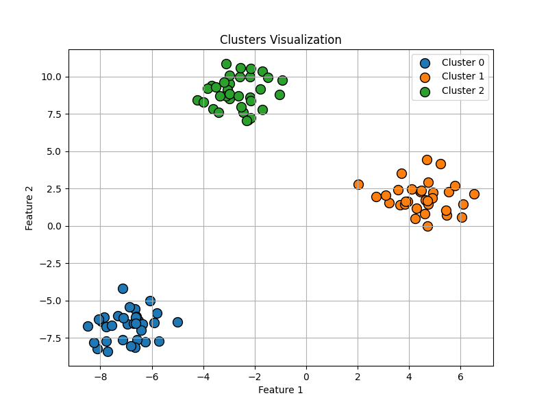
clusters = hierarchical_clustering(data, threshold=threshold)

In the code, we first generate a synthetic dataset using the make_blobs() function from sklearn.datasets. This function creates 100 data points (n_samples=100) grouped around 3 distinct cluster centers (centers=3) with a standard deviation of 1.0 for each cluster (cluster_std=1.0).

After generating the data, we define a distance threshold of 2.0, which will be used in the hierarchical clustering algorithm. We then call the hierarchical_clustering() function with the generated data and the specified threshold. The function groups data points into clusters based on whether the pairwise distances between points are below this threshold.

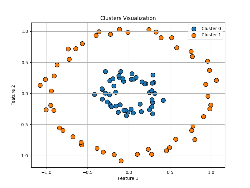
Next, let’s explore another well-known example often used in testing clustering algorithms: the dataset generated by the make_circles() function. This function creates a set of data points arranged in two concentric circles, which introduces a more challenging scenario for clustering algorithms. Unlike the clear separation seen in the previous example with make_blobs(), make_circles() presents overlapping regions and non-linearly separable clusters, making it an excellent test for evaluating the robustness and accuracy of clustering methods.

Python

data = make_circles(
    n_samples=100,
    noise=0.05,
    random_state=42,
    factor=0.3
)[0]
threshold = 0.3
clusters = hierarchical_clustering(data, threshold=threshold)

Similarly to the previous example, we generated a dataset of 100 points arranged in two concentric circles (n_samples=100). In this test case, we set the threshold to 0.3. It’s important to note that the threshold value is not static across different data distributions and must be adjusted through trial and error to find an appropriate value for each specific dataset.

Although the algorithm successfully identified the clusters in our examples, it’s worth noting that it may not always be the best choice for more complex, non-linearly separable data, such as concentric circles. Each clustering algorithm has its own strengths and weaknesses, and fine-tuning parameters can often yield better results depending on the dataset. However, for the purposes of this blog post, we focused on simpler, well-structured data to demonstrate the implementation effectively.

Performance Comparison

In conclusion, we’ll evaluate how the naive approach and the union-find-based approach perform when benchmarked across datasets of varying sizes. The naive method works by repeatedly merging the closest pair of clusters until only one cluster remains. In this brute-force approach, the algorithm recalculates the minimum distances between clusters at each step, making it computationally expensive as the dataset grows. On the other hand, the union-find structure optimizes this process by efficiently managing the merging of clusters and reducing the need for redundant distance calculations. This comparison will help highlight the trade-offs between simplicity and scalability in clustering algorithms.

def single_linkage_clustering_naive(data, threshold):
    n = len(data)
    clusters = [[i] for i in range(n)]

    distances = pdist(data)
    dist_matrix = squareform(distances)

    while len(clusters) > 1:
        min_distance = float('inf')
        clusters_to_merge = (None, None)

        for i in range(len(clusters)):
            for j in range(i + 1, len(clusters)):

                for point_i in clusters[i]:
                    for point_j in clusters[j]:
                        if dist_matrix[point_i][point_j] < min_distance:
                            min_distance = dist_matrix[point_i][point_j]
                            clusters_to_merge = (i, j)


        if min_distance > threshold:
            break

        i, j = clusters_to_merge
        clusters[i].extend(clusters[j])
        del clusters[j]

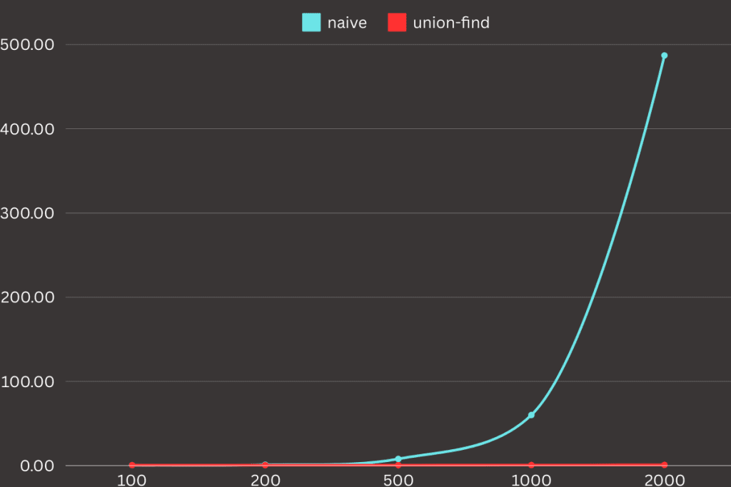
    return clusters

I conducted a small experiment using datasets of varying sizes: 100, 200, 500, 1000, and 2000 points. Both the naive and union-find implementations were tested with identical parameters, ensuring consistent conditions across all experiments. To measure the execution time, I used the time command, which provided a clear comparison of the performance between the two approaches as the dataset sizes increased.

Bash

time python script.py

>> python script.py  0.88s user 0.13s system 92% cpu 1.100 total

Based on the results of the experiment, it is clear that the union-find-based approach significantly outperforms the naive implementation as dataset sizes increase. For smaller datasets (100 and 200 points), the execution times between the two methods are relatively similar, with the naive method slightly slower. However, as the dataset size grows, the naive approach becomes exponentially slower, taking nearly 8 seconds for 500 points and over 8 minutes for 2000 points. In contrast, the union-find approach remains consistently efficient, with execution times barely increasing even for the largest dataset.

This demonstrates that selecting the right data structure for a given task can play a crucial role in optimizing execution time. In this case, the union-find structure dramatically improved performance, reducing processing time from hours to just minutes or even seconds. This principle applies not only to clustering algorithms but to problem-solving in general: a well-chosen algorithm or structure can drastically increase efficiency, making a significant difference in both development time and computational resources.

Summary

In conclusion, the union-find data structure has proven to be a highly effective tool for handling various clustering tasks. By streamlining operations such as merging clusters and efficiently managing connectivity checks, union-find significantly enhances the performance of algorithms like hierarchical clustering. Its ability to dynamically merge points into clusters while maintaining minimal computational overhead makes it particularly well-suited for large datasets.

This blog post specifically focused on the application of union-find in clustering algorithms, highlighting how it effectively manages dynamic cluster formation in approaches such as single-linkage clustering. The flexibility of the union-find structure enables it to adapt well to diverse datasets, offering significant improvements in terms of speed and scalability. By leveraging union-find, we eliminate redundant calculations and ensure faster convergence in clustering tasks.

Beyond clustering, the utility of union-find extends to a wide range of graph-based problems. Its adaptability and efficiency make it an invaluable tool for solving complex data structure challenges in multiple domains, further solidifying its importance in modern algorithmic solutions.