
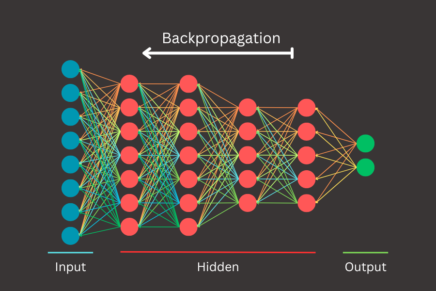
Artificial intelligence (AI) has rapidly advanced, transforming industries and pushing technological boundaries. Central to this progress is backpropagation, the essential algorithm that enables neural networks to learn and adapt. Often considered the heartbeat of AI, backpropagation drives the learning process, allowing machines to improve with experience. In this blog post, we’ll demystify backpropagation, exploring its mathematical foundations and practical implementation. Whether you’re an experienced machine learning practitioner or a curious beginner, this deep dive will not only shed light on the algorithms powering intelligent systems but also enhance your understanding step by step.
Backprop or how to learn
Backpropagation works by computing the gradient of the loss function with respect to each weight by the chain rule, allowing for the systematic adjustment of weights to minimize the error. It transformed neural networks from theoretical constructs into practical tools capable of learning from data. By enabling the training of deep networks, backpropagation made it possible to tackle complex tasks that were previously out of reach, such as image and speech recognition. This breakthrough laid the foundation for the field of deep learning, which has since driven remarkable advancements across various domains of artificial intelligence.
Today, deep learning is at the heart of numerous AI applications, from self-driving cars and virtual assistants to medical diagnosis and financial forecasting. The success of these applications owes much to the power of backpropagation, which remains a cornerstone of neural network training. As we delve deeper into the mechanics of backpropagation in this blog post, we will explore its mathematical foundations and practical implementation.
To truly grasp the backpropagation algorithm, it’s essential to first understand one of its core concepts; derivatives. Derivatives measure how a function changes as its input changes, providing the sensitivity analysis needed to optimize neural network weights. By understanding derivatives, we can unlock the mechanics of how backpropagation fine-tunes neural networks to learn from data effectively.
Understanding Derivatives
In strictly mathematical terms, the derivative of function f(x) at a point x is defined as the limit of the average rate of change of the function as the interval over which the change is measured approaches to zero. Formally, the derive f'(x) is given by:

So what is intuitively derivative? Imagine you’re driving a car on a winding road through the hills. You have a GPS that shows your current elevation of the road as you drive. If you plot your journey on a graph where the x-axis represents the distance traveled and the y-axis elevation, the derivative at any point on this graph tells you the slope of the road at that exact location, the derivative tells you how steep the trail is at any given point. If the slope is steep, the elevation changes quickly, and if the slope is gentle, the elevation changes slowly.

- Steep Sections: The elevation increases rapidly, resulting in a large and positive derivative, indicating a steep upward slope
- Gentle Slopes: The elevation changes slowly, leading to a small derivative, indicating a gradual incline or decline
- Flat Sections: The elevation remains constant, producing a zero derivative, indicating no change in elevation: The elevation remains constant, producing a zero derivative, indicating no change in elevation
Multivariate Madness: When One Variable Just Isn’t Enough
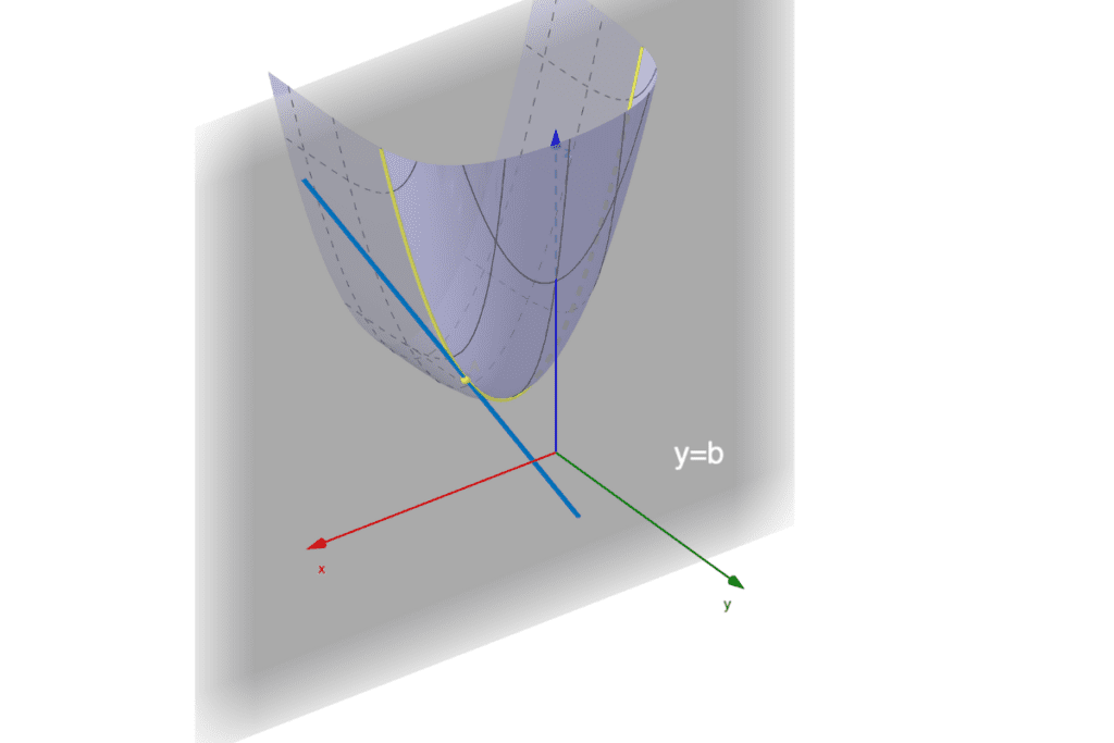
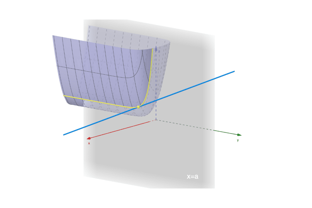
Although our initial definition of the derivative involved a function with a single variable, the concept extends to functions with multiple variables. For a function f(x1, x2, . . . , xn) ,the derivative is defined as follows:

This definition tells us that a partial derivative measures the rate of change of the function f with respect to one variable (xi) while keeping all other variables constant. In other words, it shows how f changes as one specific variable varies, isolating the effect of that variable on the function’s behavior.
The derivation introduced in this section is known as the first derivative and is typically denoted with a prime symbol, such as f’ . For multivariable functions, it is necessary to specify the variable with respect to which the derivative is taken, using notation like ∂f/∂x. In vector notation, the derivative is represented as the gradient, denoted by ∇f or ∂f/∂x , which is a vector of partial derivatives. In matrix notation, the Jacobian matrix J contains all first-order partial derivatives of a vector-valued function, while the Hessian matrix H includes second-order partial derivatives, providing a comprehensive view of the function’s curvature.
Rules of derivative
Common rules for function differentiation are derived from the limit definition, providing a solid foundation for applying these rules to a wide range of functions. This foundational approach makes it easier to handle more complex functions, such as those encountered in neural networks, where differentiation is crucial for optimization algorithms like backpropagation. By understanding these basic principles, we can effectively compute gradients, which are essential for training and fine-tuning neural network models.
| Function | Derivative |
|---|---|
| c (const) | 0 |
| x | 1 |
| cx | c |
| xn | nxn-1 |
| ex | ex |
| ln(x) | 1/x |
| ax | axln(x) |
| sin(x) | cos(x) |
| cos(x) | -sin(x) |
In addition to the basic rules for differentiating functions, there are also rules for differentiating more complex expressions involving sums, differences, products, and quotients. These rules allow us to break down and manage the differentiation of more intricate mathematical expressions, making it possible to tackle a wide variety of problems in calculus. By understanding and applying these advanced differentiation techniques, we can gain deeper insights into the behavior of functions and their rates of change.
| Rule | Derivation |
|---|---|
| (f+g)’ | f’ + g’ |
| (f-g)’ | f’ – g’ |
| (f*g)’ | f’ * g + f * g’ |
| (f/g)’ | (f’ * g – f * g’)/g2 |
| f(g(x)) | f'(g(x)) g'(x) |
Let’s gain an understanding of how to apply these rules. In this section, won’t go too deeply, but it should provide a basic sense of how the derivation is computed.
Fun with Examples
First, we applied the sum rule twice. In the first step, we grouped the first two terms together as f (according to our table of rules) and treated the last term as g . Since f itself is a sum of two terms, we applied the sum rule again to f . After breaking down the expression, we had each term ready for differentiation. At this point, we applied the specific differentiation rules for each term according to our table of function derivatives.
![\left[ \exp(x) + \sin(x) +x^2 \right]^\prime=\left[ \exp(x)^\prime + \sin(x)^\prime + (x^2)^\prime \right] = \left[ \exp(x) + \cos(x) + 2x \right]](https://s0.wp.com/latex.php?latex=%5Cleft%5B+%5Cexp%28x%29+%2B+%5Csin%28x%29+%2Bx%5E2+%5Cright%5D%5E%5Cprime%3D%5Cleft%5B+%5Cexp%28x%29%5E%5Cprime+%2B+%5Csin%28x%29%5E%5Cprime+%2B+%28x%5E2%29%5E%5Cprime+%5Cright%5D+%3D+%5Cleft%5B+%5Cexp%28x%29+%2B+%5Ccos%28x%29+%2B+2x+%5Cright%5D&bg=ffffff&fg=000&s=2&c=20201002)
To find the derivative of the sigmoid function using the quotient rule, we first identify the numerator and denominator functions. Let’s denote the numerator as f and the denominator as g . Then, we apply the quotient rule to these functions and differentiate each term accordingly based on standard differentiation rules. This expression can be simplified further, but we will leave it in its current form for clarity.
![\left[\frac{1}{1+\exp(-x)}\right]^\prime = \frac{1^\prime (1+\exp(-x)) - 1(1+exp(-x))^\prime}{(1+\exp(-x))^2} =\frac{0(1+\exp(-x)) - (-\exp(-x))}{(1+\exp(-x))^2} = \frac{\exp(-x)}{(1+\exp(-x))^2}](https://s0.wp.com/latex.php?latex=%5Cleft%5B%5Cfrac%7B1%7D%7B1%2B%5Cexp%28-x%29%7D%5Cright%5D%5E%5Cprime+%3D+%5Cfrac%7B1%5E%5Cprime+%281%2B%5Cexp%28-x%29%29+-+1%281%2Bexp%28-x%29%29%5E%5Cprime%7D%7B%281%2B%5Cexp%28-x%29%29%5E2%7D+%3D%5Cfrac%7B0%281%2B%5Cexp%28-x%29%29+-+%28-%5Cexp%28-x%29%29%7D%7B%281%2B%5Cexp%28-x%29%29%5E2%7D+%3D+%5Cfrac%7B%5Cexp%28-x%29%7D%7B%281%2B%5Cexp%28-x%29%29%5E2%7D&bg=ffffff&fg=000&s=2&c=20201002)
Chain rule
Among the rules and properties that derivatives satisfy, the chain rule stands out as one of the most useful and subtle in understanding a derivative’s behavior with respect to the composition of functions. The composition of functions occurs when one function is applied to the result of another function, creating a chain of functions. For example, if we have two functions f(x) and g(x) , their composition is denoted as f(g(x)) or (f∘g)(x). The chain rule allows us to differentiate such composite functions efficiently by taking the derivative of the outer function evaluated at the inner function and multiplying it by the derivative of the inner function. This is precisely the process used in the forward pass of a neural network, where layers of functions are composed to process inputs and generate outputs.
The chain rule may be straightforward to derive, but before we visualize it graphically, let’s work through a few examples to build intuition behind this process.
The Single Variable Saga

Here we have a composition of two functions: f depends on the variable x , which in turn is a function of the variable t. To compute the derivative of the composite function (f ∘ x) with respect to t , we need to apply the chain rule. This involves multiplying the derivative of f with respect to x by the derivative of x with respect to t , which is the composite rule described in Table 2.
Simply put, the chain rule says that if we have a function f that is differentiable at x and another function g that is differentiable at t, then we can find the derivative of their composition (f ∘ g) using the following relationship:

This graphical representation (Figure 6) of functions and the derivation of the chain rule from it play an important role here. Regardless of how many variables are involved across functions, we can model it in such a way to derive the chain rule expression. This approach will be easier to understand as we explore a few more examples from this point onward.
Tackling Two Variables

Here, we have a function f that depends at an intermediate level on two variables, x and y (or on the vector variable x = (x, y) ). This requires the use of partial derivatives. At the final level, f depends on a single variable, t . In our example, we applied the quotient rule to obtain the final result. However, using the chain rule, we generally need to work with smaller, more manageable chunks of the function to compute the derivatives.
In this case, if we have a function f that is differentiable with respect to (x, y) and a function x that is differentiable with respect to t , then we can express their relationship as follows:

The graphical representation in Figure 7 resembles the one in Figure 6, which dealt with single-variable functions at each layer. From this figure, we can already infer how to model any function with any number of variables across multiple layers. The derivative of f with respect to t is computed by considering the partial derivatives of f with respect to x and y , as well as the derivatives of x and y with respect to t.
The General Case Extravaganza
Now, if we apply the concepts learned from the previous case of functions with two variables to our example, we will achieve the same results. By computing smaller chunks of derivatives across the expression using the chain rule, we simplify the process and obtain the same outcome as when we applied the quotient rule.
The chain rule is particularly advantageous in such situations because it breaks down complex differentiation into manageable steps, making it easier to handle functions with multiple variables.
Moving forward, we can develop a more general approach for computing derivatives across various functions and layers of variables, as shown in Figure 8. If you look closely at Figure 8, it closely resembles the structure of neural networks with different numbers of layers and sizes.
In general, if we want to compute the partial derivatives of the function f1 with respect to t1 we sum the products of the derivatives along each path from f1 to t1 . This involves multiplying the partial derivatives of f1 with respect to each intermediate variable xi by the derivatives of xi with respect to t1 , and then summing these products. In a similar manner, we can compute other derivatives with respect to any variable and any function.
A Detailed Walkthrough
The process of updating weights in any neural network is given by the following expression. This expression allows us to adjust the weights to minimize the error between the predicted and actual outputs. By iteratively applying this update rule, we can train the neural network to improve its performance over time,

where Wnew is the updated weights, Wold is the current weight, η is the learning rate and dC/dW is the partial derivative of the loss function C with respect to the weight W.
The cost function we will use is the mean squared error (MSE), which measures the average of the squares of the errors between the predicted and actual values. Here a factor of 1/2 is included instead of 1/n to simplify the derivative calculations during the backpropagation process, as it cancels out the 2 that appears when differentiating the squared terms.

Let’s familiarize with some notations that will be used in this blog post. These notations will provide a clear understanding of what they represent at each step of the process.
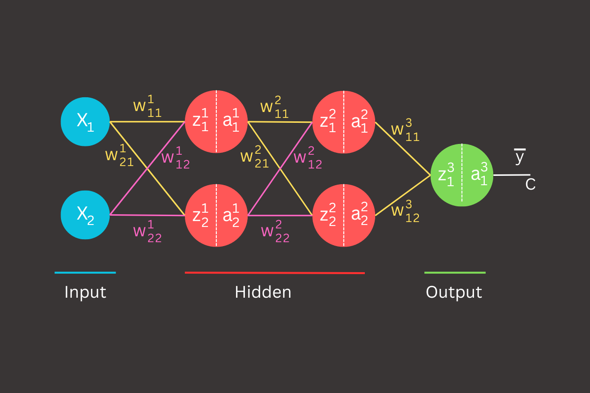
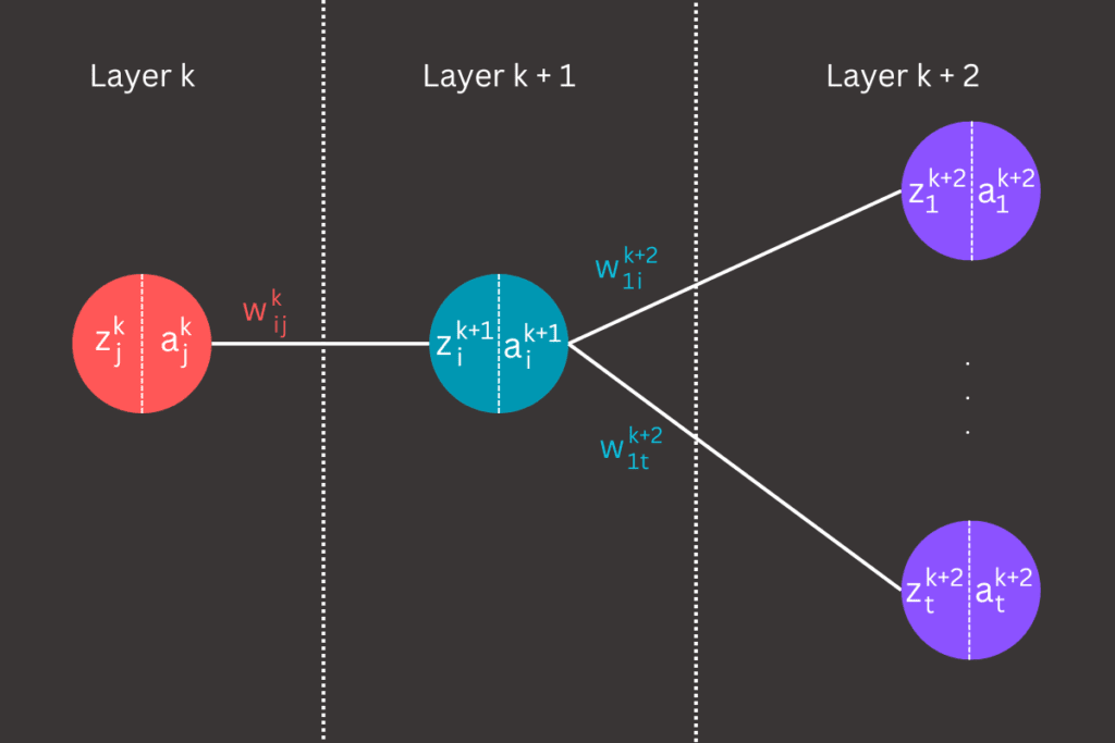

The weight w represents the connection between node j in layer k and node i in the subsequent layer k+1 . This weight determines the strength and direction of the signal that is passed from one node to the next, playing a crucial role in the learning process of the neural network. Each weight is adjusted during training to minimize the cost function and improve the accuracy of the model.

The linear term z represents a linear combination of the weights and the activation terms from the previous layer. Specifically, it is calculated as the sum of the products of the weights and the corresponding activations from the preceding layer, along with a bias term (in our example we will ignore bias term). This linear combination serves as the input to the activation function, which then introduces non-linearity into the model, enabling the neural network to capture complex patterns and relationships in the data.

The activation term a represents the result of applying the activation function to the linear term z . This process introduces non-linearity into the model by transforming the linear combination of inputs into a non-linear output. The activation function can be any non-linear function, such as the sigmoid, tanh, ReLU etc. This non-linear transformation is crucial as it enables the neural network to learn and represent complex patterns in the data.

Before we proceed with the feedforward and backpropagation processes, we need to initialize the weights in the neural network. While there are various methods to properly initialize neural network weights, in our case, we will initialize all weights in each layer to 0.5. This simplification allows us to focus on understanding the learning process without the complexities of different initialization strategies.
Chain rule them all
As outlined, updating the weights is done by subtracting the derivative of the cost function C with respect to each specific weight. In our case, the following expressions will perform this task.


To compute the derivatives of the cost function C with respect to a weight, we need to apply the same logic used in the rules of derivatives section, along with the chain rule method. In our case, the cost function C is treated as the dependent variable, while the specific weight is the final variable. All variables in the path between these two are considered intermediate variables. Along this path, we primarily encounter two types of variables: the linear term (z) and the activation function (a). To simplify the computation, we will focus on the linear term (z) and exclude the activation function (a). Additionally, we will not explicitly take derivatives of weights along the path, because the weights are constant with respect to the intermediate variables, and the chain rule allows us to focus on how changes in the activations and linear terms propagate through the network.
Referring to Figure 11, we now have the final expression for the derivatives of the cost function with respect to the weights w11 and w12 in layer 3 (the output layer). The next step is to determine the derivatives for each term in the final expression. This is a more manageable task compared to the original problem.
![\frac{\partial z_{1}^{3}}{\partial w_{11}^{3}} = \frac{\partial}{\partial w_{11}^{3}}(w_{11}^{3}a_{1}^{2}+w_{12}^{3}a_{2}^{2})=a_{1}^{2} \\ \frac{\partial z_{2}^{3}}{\partial w_{12}^{3}} = \frac{\partial}{\partial w_{12}^{3}}(w_{11}^{3}a_{1}^{2}+w_{12}^{3}a_{2}^{2}) = a_{2}^{2} \\ \frac{\partial C}{\partial z_{1}^{3}} = \frac{\partial}{\partial z_{1}^{3}}[\frac{1}{2}(y - \widehat y)^{2}] = \frac{\partial}{\partial z_{1}^{3}}[\frac{1}{2}(z_{1}^{3} - \widehat y)^{2}] = z_{1}^{3}-\widehat y](https://s0.wp.com/latex.php?latex=%5Cfrac%7B%5Cpartial+z_%7B1%7D%5E%7B3%7D%7D%7B%5Cpartial+w_%7B11%7D%5E%7B3%7D%7D+%3D+%5Cfrac%7B%5Cpartial%7D%7B%5Cpartial+w_%7B11%7D%5E%7B3%7D%7D%28w_%7B11%7D%5E%7B3%7Da_%7B1%7D%5E%7B2%7D%2Bw_%7B12%7D%5E%7B3%7Da_%7B2%7D%5E%7B2%7D%29%3Da_%7B1%7D%5E%7B2%7D+%5C%5C+%5Cfrac%7B%5Cpartial+z_%7B2%7D%5E%7B3%7D%7D%7B%5Cpartial+w_%7B12%7D%5E%7B3%7D%7D+%3D+%5Cfrac%7B%5Cpartial%7D%7B%5Cpartial+w_%7B12%7D%5E%7B3%7D%7D%28w_%7B11%7D%5E%7B3%7Da_%7B1%7D%5E%7B2%7D%2Bw_%7B12%7D%5E%7B3%7Da_%7B2%7D%5E%7B2%7D%29+%3D+a_%7B2%7D%5E%7B2%7D+%5C%5C+%5Cfrac%7B%5Cpartial+C%7D%7B%5Cpartial+z_%7B1%7D%5E%7B3%7D%7D+%3D+%5Cfrac%7B%5Cpartial%7D%7B%5Cpartial+z_%7B1%7D%5E%7B3%7D%7D%5B%5Cfrac%7B1%7D%7B2%7D%28y+-+%5Cwidehat+y%29%5E%7B2%7D%5D+%3D+%5Cfrac%7B%5Cpartial%7D%7B%5Cpartial+z_%7B1%7D%5E%7B3%7D%7D%5B%5Cfrac%7B1%7D%7B2%7D%28z_%7B1%7D%5E%7B3%7D+-+%5Cwidehat+y%29%5E%7B2%7D%5D+%3D+z_%7B1%7D%5E%7B3%7D-%5Cwidehat+y&bg=ffffff&fg=000&s=2&c=20201002)
Once the terms are computed, we can simply plug them into the expressions shown in Figure 11. This will allow us to compute the final derivatives with respect to w11 and w12 .

By following the same method and applying the chain rule in layer 2, we can derive the expressions for the derivatives of the cost function C with respect to the weights w11, w12, w21, and w22. This computation is shown in Figure 12.

We began by computing the rightmost terms in the expressions, focusing on the derivatives of the linear terms with respect to the weights. These are fairly easy to obtain because they represent direct linear sums of the activation terms.
![\frac{\partial z_{1}^{3}}{\partial z_{1}^{2}} = \frac{\partial}{\partial z_{1}^{2}}(w_{11}^{3}a_{1}^{2} + w_{12}^{3}a_{2}^{2}) = \frac{\partial}{\partial z_{1}^{2}}[w_{11}^{3}h(z_{1}^{2}) + w_{12}^{3}h(z_{2}^{2})] = w_{11}^{3}h^{\prime}(z_{1}^{2}) \\ \frac{\partial z_{1}^{3}}{\partial z_{2}^{2}} = w_{12}^{3}h^{\prime}(z_{2}^{2})](https://s0.wp.com/latex.php?latex=%5Cfrac%7B%5Cpartial+z_%7B1%7D%5E%7B3%7D%7D%7B%5Cpartial+z_%7B1%7D%5E%7B2%7D%7D+%3D+%5Cfrac%7B%5Cpartial%7D%7B%5Cpartial+z_%7B1%7D%5E%7B2%7D%7D%28w_%7B11%7D%5E%7B3%7Da_%7B1%7D%5E%7B2%7D+%2B+w_%7B12%7D%5E%7B3%7Da_%7B2%7D%5E%7B2%7D%29+%3D+%5Cfrac%7B%5Cpartial%7D%7B%5Cpartial+z_%7B1%7D%5E%7B2%7D%7D%5Bw_%7B11%7D%5E%7B3%7Dh%28z_%7B1%7D%5E%7B2%7D%29+%2B+w_%7B12%7D%5E%7B3%7Dh%28z_%7B2%7D%5E%7B2%7D%29%5D+%3D+w_%7B11%7D%5E%7B3%7Dh%5E%7B%5Cprime%7D%28z_%7B1%7D%5E%7B2%7D%29+%5C%5C+%5Cfrac%7B%5Cpartial+z_%7B1%7D%5E%7B3%7D%7D%7B%5Cpartial+z_%7B2%7D%5E%7B2%7D%7D+%3D+w_%7B12%7D%5E%7B3%7Dh%5E%7B%5Cprime%7D%28z_%7B2%7D%5E%7B2%7D%29&bg=ffffff&fg=000&s=2&c=20201002)
In our next steps, we computed derivatives reflecting the sensitivity of the output linear combination to changes in the input activations. This process didn’t introduce any new concepts; thus, computing the final derivatives requires replacing the activation terms with the corresponding linear terms, which the activation functions take as arguments. We then follow the rules introduced in the derivatives section to complete the computation.


Note that the final term we computed in the previous layer is the derivative of the cost function C with respect to the linear terms z1 in layer 3 (the output layer).

By repeating the same procedure, let’s compute the derivatives of the linear terms with respect to the weights.


Next, we compute the derivatives that reflect the sensitivity of the output linear combination to changes in the input activations, within the context of the layer where we are performing the derivative calculations.


Note that some terms have already been computed in the previous layer, so we can simply plug them into the expression to obtain the required derivatives.

By plugging all the terms into the expressions derived in Figure 13, we obtain the final set of derivatives, which can be used in the backpropagation process to update the weights. It is important to note that as we step back to layer 1, a significant amount of computation can be reused from the previous layer, as many terms reappear repeatedly. This is beneficial not only for manual calculation but also for implementation in code.
This memoization technique helps speed up the processing of neural networks, which often contain millions of parameters for specific tasks. The function h(x) in a neural network is the activation function, which is selected before the training process begins. It can be configured to be used globally across all layers or set to different activation functions for specific layers.


For example, let’s consider a data point with x1 = 1, x2 = 1, and y = 1.5. We perform the feedforward process with all weights initialized to 0.5, and we use the ReLU function as the activation function in the first two layers (layer 1 and layer 2).
Layer 1

Layer 2

Layer 3 (output)

The backpropagation process is straightforward because we have the necessary derivatives ready for use in updating the weights. The parameter η, known as the learning rate, is defined before the training process begins. It controls the size of the steps taken during the optimization process.
Layer 1 weight update process
![w_{11}^1 = w_{11}^1 - \eta \frac{\partial C}{\partial w_{11}^1} = 0.5 - \eta [(z_{1}^{3}-\widehat y)w_{11}^{3}h^{\prime}(z_{1}^{2})w_{11}^{2}h^{\prime}(z_{1}^{1})x_{1} + (z_{1}^{3}-\widehat y)w_{12}^{3}h^{\prime}(z_{2}^{2})w_{21}^{2}h^{\prime}(z_{1}^{1})x_{1} ] = 0.5 - \eta [(1.0 - 1.5) \cdot 0.5 \cdot 1.0 \cdot 0.5 \cdot 1.0 \cdot 1.0 + (1.0 - 1.5) \cdot 0.5 \cdot 1.0 \cdot 0.5 \cdot 1.0 \cdot 1.0] \\ w_{12} ^ 1 = w_{12} ^ 1 - \eta \frac{\partial C}{\partial w_{12}^1} = w_{12}^1 - \eta [(z_{1}^{3}-\widehat y)w_{11}^{3}h^{\prime}(z_{1}^{2})w_{11}^{2}h^{\prime}(z_{1}^{1})x_{2} + (z_{1}^{3}-\widehat y)w_{12}^{3}h^{\prime}(z_{2}^{2})w_{21}^{2}h^{\prime}(z_{1}^{1})x_{2}] = 0.5 - \eta [(1.0 - 1.5) \cdot 0.5 \cdot 1.0 \cdot 0.5 \cdot 1.0 \cdot 1.0 + (1.0 - 1.5) \cdot 0.5 \cdot 1.0 \cdot 0.5 \cdot 1.0 \cdot 1.0]](https://s0.wp.com/latex.php?latex=w_%7B11%7D%5E1+%3D+w_%7B11%7D%5E1+-+%5Ceta+%5Cfrac%7B%5Cpartial+C%7D%7B%5Cpartial+w_%7B11%7D%5E1%7D+%3D+0.5+-+%5Ceta+%5B%28z_%7B1%7D%5E%7B3%7D-%5Cwidehat+y%29w_%7B11%7D%5E%7B3%7Dh%5E%7B%5Cprime%7D%28z_%7B1%7D%5E%7B2%7D%29w_%7B11%7D%5E%7B2%7Dh%5E%7B%5Cprime%7D%28z_%7B1%7D%5E%7B1%7D%29x_%7B1%7D+%2B+%28z_%7B1%7D%5E%7B3%7D-%5Cwidehat+y%29w_%7B12%7D%5E%7B3%7Dh%5E%7B%5Cprime%7D%28z_%7B2%7D%5E%7B2%7D%29w_%7B21%7D%5E%7B2%7Dh%5E%7B%5Cprime%7D%28z_%7B1%7D%5E%7B1%7D%29x_%7B1%7D+%5D+%3D+0.5+-+%5Ceta+%5B%281.0+-+1.5%29+%5Ccdot+0.5+%5Ccdot+1.0+%5Ccdot+0.5+%5Ccdot+1.0+%5Ccdot+1.0+%2B+%281.0+-+1.5%29+%5Ccdot+0.5+%5Ccdot+1.0+%5Ccdot+0.5+%5Ccdot+1.0+%5Ccdot+1.0%5D+%5C%5C+w_%7B12%7D+%5E+1+%3D+w_%7B12%7D+%5E+1+-+%5Ceta+%5Cfrac%7B%5Cpartial+C%7D%7B%5Cpartial+w_%7B12%7D%5E1%7D+%3D+w_%7B12%7D%5E1+-+%5Ceta+%5B%28z_%7B1%7D%5E%7B3%7D-%5Cwidehat+y%29w_%7B11%7D%5E%7B3%7Dh%5E%7B%5Cprime%7D%28z_%7B1%7D%5E%7B2%7D%29w_%7B11%7D%5E%7B2%7Dh%5E%7B%5Cprime%7D%28z_%7B1%7D%5E%7B1%7D%29x_%7B2%7D+%2B+%28z_%7B1%7D%5E%7B3%7D-%5Cwidehat+y%29w_%7B12%7D%5E%7B3%7Dh%5E%7B%5Cprime%7D%28z_%7B2%7D%5E%7B2%7D%29w_%7B21%7D%5E%7B2%7Dh%5E%7B%5Cprime%7D%28z_%7B1%7D%5E%7B1%7D%29x_%7B2%7D%5D+%3D+0.5+-+%5Ceta+%5B%281.0+-+1.5%29+%5Ccdot+0.5+%5Ccdot+1.0+%5Ccdot+0.5+%5Ccdot+1.0+%5Ccdot+1.0+%2B+%281.0+-+1.5%29+%5Ccdot+0.5+%5Ccdot+1.0+%5Ccdot+0.5+%5Ccdot+1.0+%5Ccdot+1.0%5D&bg=ffffff&fg=000&s=2&c=20201002)
![w_{21}^1 = w_{21}^1 - \eta \frac{\partial C}{\partial w_{21}^1} = 0.5 - \eta [(z_{1}^{3}-\widehat y)w_{11}^{3}h^{\prime}(z_{1}^{2})w_{12}^{2}h^{\prime}(z_{2}^{1})x_{1} + (z_{1}^{3}-\widehat y)w_{12}^{3}h^{\prime}(z_{2}^{2})w_{22}^{2}h^{\prime}(z_{2}^{1})x_{1}] = 0.5 - \eta[(1.0 - 1.5) \cdot 0.5 \cdot 1.0 \cdot 0.5 \cdot 1.0 \cdot 1.0 + (1.0 - 1.5) \cdot 0.5 \cdot 1.0 \cdot 0.5 \cdot 1.0 \cdot 1.0] \\ w_{22}^1 = w_{22}^1 - \eta \frac{\partial C}{\partial w_{22}^1} = w_{22}^1 - \eta [(z_{1}^{3}-\widehat y)w_{11}^{3}h^{\prime}(z_{1}^{2})w_{12}^{2}h^{\prime}(z_{2}^{1})x_{2} + (z_{1}^{3}-\widehat y)w_{12}^{3}h^{\prime}(z_{2}^{2})w_{22}^{2}h^{\prime}(z_{2}^{1})x_{2}] = 0.5 - \eta [(1.0 - 1.5) \cdot 0.5 \cdot 1.0 \cdot 0.5 \cdot 1.0 \cdot 1.0 + (1.0 - 1.5) \cdot 0.5 \cdot 1.0 \cdot 0.5 \cdot 1.0 \cdot 1.0]](https://s0.wp.com/latex.php?latex=w_%7B21%7D%5E1+%3D+w_%7B21%7D%5E1+-+%5Ceta+%5Cfrac%7B%5Cpartial+C%7D%7B%5Cpartial+w_%7B21%7D%5E1%7D+%3D+0.5+-+%5Ceta+%5B%28z_%7B1%7D%5E%7B3%7D-%5Cwidehat+y%29w_%7B11%7D%5E%7B3%7Dh%5E%7B%5Cprime%7D%28z_%7B1%7D%5E%7B2%7D%29w_%7B12%7D%5E%7B2%7Dh%5E%7B%5Cprime%7D%28z_%7B2%7D%5E%7B1%7D%29x_%7B1%7D+%2B+%28z_%7B1%7D%5E%7B3%7D-%5Cwidehat+y%29w_%7B12%7D%5E%7B3%7Dh%5E%7B%5Cprime%7D%28z_%7B2%7D%5E%7B2%7D%29w_%7B22%7D%5E%7B2%7Dh%5E%7B%5Cprime%7D%28z_%7B2%7D%5E%7B1%7D%29x_%7B1%7D%5D+%3D+0.5+-+%5Ceta%5B%281.0+-+1.5%29+%5Ccdot+0.5+%5Ccdot+1.0+%5Ccdot+0.5+%5Ccdot+1.0+%5Ccdot+1.0+%2B+%281.0+-+1.5%29+%5Ccdot+0.5+%5Ccdot+1.0+%5Ccdot+0.5+%5Ccdot+1.0+%5Ccdot+1.0%5D+%5C%5C+w_%7B22%7D%5E1+%3D+w_%7B22%7D%5E1+-+%5Ceta+%5Cfrac%7B%5Cpartial+C%7D%7B%5Cpartial+w_%7B22%7D%5E1%7D+%3D+w_%7B22%7D%5E1+-+%5Ceta+%5B%28z_%7B1%7D%5E%7B3%7D-%5Cwidehat+y%29w_%7B11%7D%5E%7B3%7Dh%5E%7B%5Cprime%7D%28z_%7B1%7D%5E%7B2%7D%29w_%7B12%7D%5E%7B2%7Dh%5E%7B%5Cprime%7D%28z_%7B2%7D%5E%7B1%7D%29x_%7B2%7D+%2B+%28z_%7B1%7D%5E%7B3%7D-%5Cwidehat+y%29w_%7B12%7D%5E%7B3%7Dh%5E%7B%5Cprime%7D%28z_%7B2%7D%5E%7B2%7D%29w_%7B22%7D%5E%7B2%7Dh%5E%7B%5Cprime%7D%28z_%7B2%7D%5E%7B1%7D%29x_%7B2%7D%5D+%3D+0.5+-+%5Ceta+%5B%281.0+-+1.5%29+%5Ccdot+0.5+%5Ccdot+1.0+%5Ccdot+0.5+%5Ccdot+1.0+%5Ccdot+1.0+%2B+%281.0+-+1.5%29+%5Ccdot+0.5+%5Ccdot+1.0+%5Ccdot+0.5+%5Ccdot+1.0+%5Ccdot+1.0%5D&bg=ffffff&fg=000&s=2&c=20201002)
Layer 2 weight update process

Layer 3 (output) weight update process

Implementing Backpropagation
In this section, we will dive straight into the implementation of the backpropagation algorithm, including an additional check to ensure the correctness of our computations.
Checking the derivatives with the limit definition is a crucial step to ensure the correctness of the backpropagation implementation. The limit definition of a derivative provides a numerical approximation by evaluating the change in the function’s output with a small perturbation in the input. This method involves slightly increasing and decreasing each weight and bias, calculating the corresponding loss, and then using these values to estimate the gradient. By comparing these numerical gradients to the analytical gradients obtained through backpropagation, we can verify the accuracy of our implementation. This comparison helps identify any discrepancies or errors in the gradient computation, ensuring that the backpropagation algorithm correctly updates the neural network’s weights and biases.
Steps to compute numerical gradient involves following steps:
- Perturb the parameter
- For each weight wij and bias bi in the neural network create perturbed versions of these parameters


- Compute loss for perturbed parameters
- Calculate the loss function C for each perturbed parameters


- Estimate numerical gradients
- Use the limit definition to estimate the gradient
- For weights and biases
- Use the limit definition to estimate the gradient


By comparing the numerical gradients computed using the above steps with the analytical gradients obtained from backpropagation, we can verify the correctness of the gradient computation. If the numerical and analytical gradients are close, typically within a threshold such as 10-5 or 10-6, it indicates that the backpropagation implementation is correct. Large discrepancies between them suggest potential errors in the gradient calculation process.
For example, for weight w11 in layer 1 and small ϵ we need to compute the loss with w11 perturbed positively and negatively:


An additional point in the implementation is the introduction of a helper variable, often referred to as node error in the literature and denoted as

This variable represents the error term for node i in the layer k, which quantifies the contribution of that node to the overall error. The node error is crucial for propagating errors backward through the network and adjusting the weights accordingly during the backpropagation process.
Computing the error term for nodes in the final (output) layer is straightforward since there are no additional dependencies in subsequent layers. For the hidden layers, the computation is derived similarly using the chain rule, as presented in section where we explained chain rule.
Output layer (L)

Hidden layers (l)

import numpy as np

# Activation functions and their derivatives
ACTIVATION_FUNCTIONS = {
    'relu': lambda x: np.maximum(0, x)
}

DERIVATIVE_ACTIVATION_FUNCTIONS = {
    'relu': lambda x: (x > 0) * 1
}


class SimpleNN:
    def __init__(self, layer_config: list[int]):
        self.num_layers = len(layer_config)
        self.layer_config = layer_config
        self.weights = [np.random.randn(y, x) for x, y in zip(layer_config[:-1], layer_config[1:])]
        self.biases = [np.random.randn(y, 1) for y in layer_config[1:]]
        self.activation_function_name = 'relu'

    def predict(self, x):
        x = x.reshape(-1, 1)
        for w, b in zip(self.weights, self.biases):
            x = ACTIVATION_FUNCTIONS[self.activation_function_name](np.dot(w, x) + b)
        return x

    def fit(self, train, labels, epochs, learning_rate=1e-2):
        train_data = np.array(train)
        label_data = np.array(labels)

        for epoch in range(epochs):
            # Shuffle the data
            indices = np.arange(len(train_data))
            np.random.shuffle(indices)
            train_data = train_data[indices]
            label_data = label_data[indices]

            for x, y in zip(train_data, label_data):
                self._backprop(x, y, learning_rate)

            if epoch % 10 == 0:
                print(f'Epoch {epoch} completed')
                total_loss = 0
                for x, y in zip(train_data, label_data):
                    mean_absolute_error = np.mean(np.abs(self.predict(x) - y))
                    total_loss += mean_absolute_error
                print(f'Loss: {total_loss / len(train_data)}')

    def _backprop(self, x, y, learning_rate):
        prime_b = [np.zeros(b.shape) for b in self.biases]
        prime_w = [np.zeros(w.shape) for w in self.weights]

        # Forward pass
        activation = x.reshape(-1, 1)
        activations = [activation]
        linear_terms = []

        for w, b in zip(self.weights, self.biases):
            z = np.dot(w, activation) + b
            linear_terms.append(z)
            activation = ACTIVATION_FUNCTIONS[self.activation_function_name](z)
            activations.append(activation)

        # Backward pass
        delta = (activations[-1] - y.reshape(-1, 1)) * DERIVATIVE_ACTIVATION_FUNCTIONS[self.activation_function_name](linear_terms[-1])
        prime_b[-1] = delta
        prime_w[-1] = np.dot(delta, activations[-2].T)

        for layer_idx in range(2, self.num_layers):
            z = linear_terms[-layer_idx]
            sp = DERIVATIVE_ACTIVATION_FUNCTIONS[self.activation_function_name](z)
            delta = np.dot(self.weights[-layer_idx + 1].T, delta) * sp
            prime_b[-layer_idx] = delta
            prime_w[-layer_idx] = np.dot(delta, activations[-layer_idx - 1].T)

        epsilon = 1e-5
        numerical_prime_w = [np.zeros(w.shape) for w in self.weights]
        numerical_prime_b = [np.zeros(b.shape) for b in self.biases]

        for layer_idx, (w, b) in enumerate(zip(self.weights, self.biases)):
            for i in range(w.shape[0]):
                for j in range(w.shape[1]):
                    w_plus = w.copy()
                    w_minus = w.copy()
                    w_plus[i, j] += epsilon
                    w_minus[i, j] -= epsilon

                    self.weights[layer_idx] = w_plus
                    loss_plus = self._compute_loss(x, y)
                    self.weights[layer_idx] = w_minus
                    loss_minus = self._compute_loss(x, y)
                    self.weights[layer_idx] = w  # Restore original weights

                    numerical_prime_w[layer_idx][i, j] = (loss_plus - loss_minus) / (2 * epsilon)

            for i in range(b.shape[0]):
                b_plus = b.copy()
                b_minus = b.copy()
                b_plus[i, 0] += epsilon
                b_minus[i, 0] -= epsilon

                self.biases[layer_idx] = b_plus
                loss_plus = self._compute_loss(x, y)
                self.biases[layer_idx] = b_minus
                loss_minus = self._compute_loss(x, y)
                self.biases[layer_idx] = b  # Restore original biases

                numerical_prime_b[layer_idx][i, 0] = (loss_plus - loss_minus) / (2 * epsilon)

        for layer_idx in range(self.num_layers - 1):
            w_diff = np.linalg.norm(prime_w[layer_idx] - numerical_prime_w[layer_idx])
            b_diff = np.linalg.norm(prime_b[layer_idx] - numerical_prime_b[layer_idx])
            print(f'Layer {layer_idx + 1} - Weight difference: {w_diff:.10f}, Bias difference: {b_diff:.10f}')

        self.weights = [w - learning_rate * nw for w, nw in zip(self.weights, prime_w)]
        self.biases = [b - learning_rate * nb for b, nb in zip(self.biases, prime_b)]

    def _compute_loss(self, x, y):
        activation = x.reshape(-1, 1)
        for w, b in zip(self.weights, self.biases):
            activation = ACTIVATION_FUNCTIONS[self.activation_function_name](np.dot(w, activation) + b)
        return np.mean((activation - y.reshape(-1, 1)) ** 2)

# Test the network with a simple configuration
layer_config = [2, 4, 1]
nn = SimpleNN(layer_config)

# Example data with multiple samples
train_data = np.array([[1, 1], [0, 1], [1, 0], [0, 0]])
label_data = np.array([[1.5], [0.5], [0.5], [0]])

# Train the network
nn.fit(train_data, label_data, epochs=1000, learning_rate=1e-2)
The code is relatively straightforward, but there are a few crucial lines that deserve special attention at the moment:
- In line 65, we compute the error term (δ) for the nodes in the output layer. This term quantifies each node’s contribution to the overall error, as stated above.
- Lines 69 to 74 iteratively compute the error term for the nodes in the hidden layers. The chain rule is applied to propagate the error backward through the network, allowing for the adjustment of weights and biases accordingly.
- Lines 76 to 113 represent an additional check for verifying our gradient computation method in the neural network. This process is slow, so to speed up the overall execution, you can comment out or remove these lines.
Conclusion
In conclusion, mastering the backpropagation algorithm is like learning to dance: it requires precision, practice, and occasionally stepping on some toes. By ensuring our gradients are correctly computed and validated with numerical checks, we can confidently lead our neural networks to better performance. Think of numerical gradient checks as our dance mirror, reflecting any missteps and helping us stay in rhythm. With these techniques, not only do we fine-tune our models, but we also gain a deeper understanding of the intricate choreography behind machine learning. So, let’s keep dancing through data, one gradient at a time. For more insights on neural networks, you can check out my previous blog post, Unlocking Neural Networks with JAX.