Unlocking Neural Networks with JAX

Welcome back to our Unlocking with JAX series! Today, we’re getting hands-on with neural networks by building a multilayer perceptron (MLP) using JAX. JAX sits perfectly between the lower-level, details of CUDA and the higher-level abstractions offered by frameworks like Keras, offering both clarity and control. This balance helps immensely in understanding the inner workings of neural networks.In this post, we’ll walk through the steps to create an neural network from the ground up. We’ll see how JAX’s features, like automatic differentiation and efficient hardware utilization, can make our life easier and our code faster. Whether you’re just starting out or you’ve been around the block, there’s something here for everyone. Ready to get started with some real coding? Let’s jump right in!

Buzzing Through Neural Network

Multilayer perceptrons (MLPs) are a fundamental type of neural network, often used as an introductory model for understanding the principles of deep learning. An MLP consists of multiple layers of nodes, which are categorized into three types:

• input layer
  • This layer receives the raw input data, each node corresponding to a feature in the data set
• one or more hidden layers
  • These intermediate layers transform inputs from the previous layer using a weighted sum followed by a non-linear (or linear) activation function. This setup allows the network to learn complex patterns and relationships in the data
• output layer
  • The final layer that produces the network’s output, which could be a class label in classification tasks or a continuous value in regression

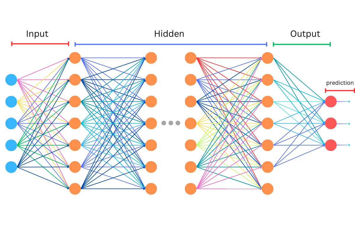
From this point and further in the text, we will use the term neural network to refer to what we have previously discussed as an MLP, ensuring consistency and clarity as we explore deeper into the subject.

So, if we look at Figure 1, we see a lot of connections between circles, and you might wonder what these represent. Each arrow or edge between two circles represents a weight that must be used in computations involving these circles. In the context of neural network, each circle represents a neuron, and the arrows show the connections through which data flows from one neuron to another. The weight on each connection modifies the signal that passes along it, based on the strength of the connection that has been learned during training.

During the process of learning, these weights are adjusted to minimize errors in output, essentially tuning the network to respond correctly to a variety of inputs. This fine-tuning occurs through a method known as backpropagation, where the network adjusts the weights in reverse, from the output back to the input, optimizing the path the data takes through the network for accurate predictions.

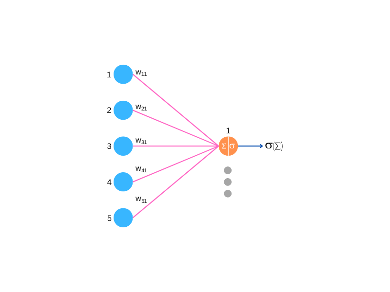
This Figure 2, shows a segment of a multilayer perceptron, representing a typical layer configuration found within these networks. While the specific layer depicted may vary, the fundamental computational process remains consistent throughout the network.

Each pink arrow in the diagram represents a weight, a key parameter that the network fine-tunes during training. These weights are vital as they adjust the strength of the input signals received by the neurons. Within the neuron, these weighted inputs are summed and then transformed by an activation function to produce the output signal, as shown by the blue arrow exiting the orange neuron.

The choice of activation function is critical. Using non-linear activation functions in these neurons, rather than linear ones, prevents the network from simplifying into a single-layer linear model, which would occur regardless of the number of layers present. This limitation is significant because it would inhibit the network’s capacity to model the complex patterns and relationships inherent in the data. Non-linear activations empower the network to learn and express more intricate functions, enhancing the model’s depth and predictive power.

A Matrix Viewpoint on Multilayer Perceptrons

In this post, we will not go into great detail about matrix operations, although it’s important to recognize them as a core concept in the deep learning world.
The architecture of neural network inherently relies on matrix multiplication to perform its operations. This method is not just a convenient mathematical approach; it is foundational for enabling efficient data processing across the network’s multiple layers. Each layer in a neural network effectively acts as a matrix of weights, with input data treated as vectors. Multiplying the input vector by the weight matrix produces a new vector, which then serves as the input to the next layer. This process of matrix multiplication consolidates the steps of weight adjustment and signal transmission into one efficient operation, dramatically accelerating computations.

Moreover, matrix multiplication is particularly well-suited to modern hardware. Computing architectures, especially those in GPUs and TPUs, are optimized to perform large-scale matrix operations very efficiently. This hardware compatibility allows neural networks to leverage parallel processing capabilities, enabling the simultaneous handling of vast datasets and complex calculations. This synergy significantly enhances performance and scalability, making matrix multiplication indispensable for high-speed neural computing.

For clarity and simplicity, let’s envision building an neural network. Imagine an neural network that features an input layer representing the number of features in our dataset, two hidden layers, and an output layer designed to learn continuous values from an imaginary dataset.

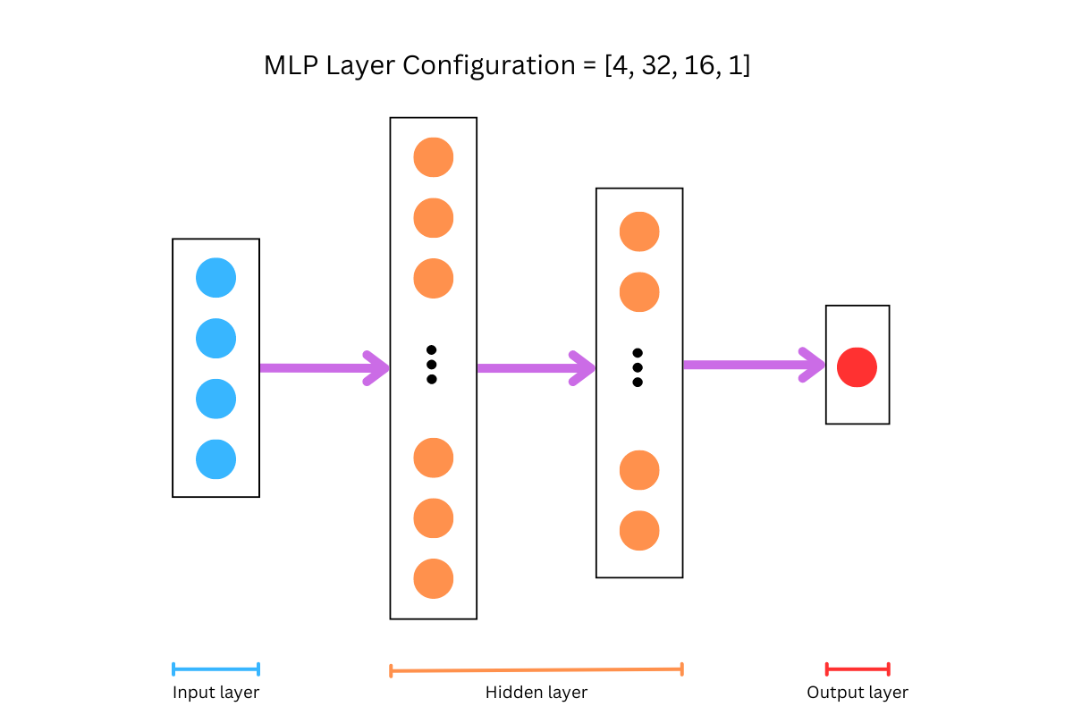
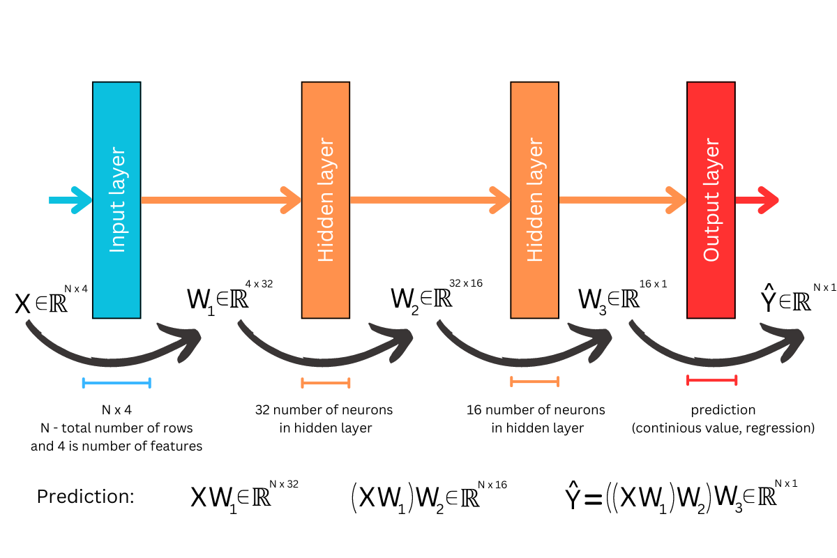
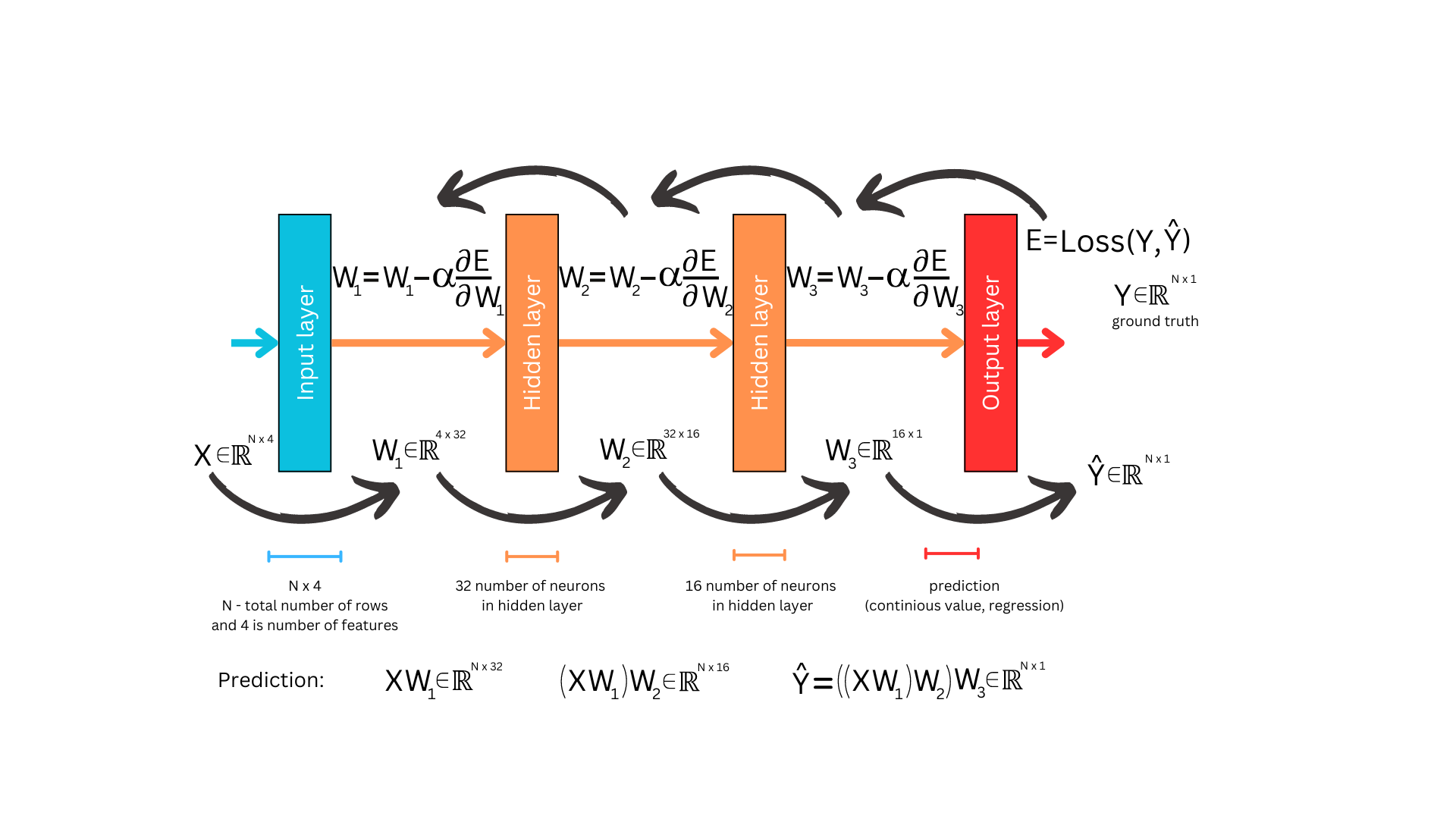
Figure 3 and Figure 4 illustrate the neural network during the feed-forward phase, also known as the prediction phase. Typically, our dataset (assuming it fits in memory) is stored as a matrix with N rows and F columns, representing the features. During the initialization phase, the network’s weights are randomly generated, but it’s crucial to ensure that the dimensions match at each step of matrix multiplication; otherwise, the computation cannot proceed. At this stage, understanding when matrix multiplication is possible—and when it isn’t—is essential.

Lets go forward

We begin with our data matrix, X, and in the first step, we use the weight matrix W₁ to calculate the activations from the first hidden layer. Note that to simplify this diagram, we omit the activation function typically applied after summing the weighted inputs. After computing XW₁, we move to the second hidden layer. Here, we perform another multiplication: (XW₁)W₂. Finally, to obtain the network’s predictions, we multiply the result from the second hidden layer with W₃, leading to Y_hat = ((XW₁)W₂)W₃. The final result is a matrix of dimensions Nx1, with each row representing a prediction corresponding to each input row fed into the neural network.

Once the prediction phase is complete, we proceed to learn from the results obtained at the output layer. The necessity for this learning phase stems from the fact that the weights of the network were initially set to random values. Since random values do not inherently contain predictive power, without learning, the output would likely be meaningless—unless one were extraordinarily lucky, which is practically impossible. The learning process is essential to refine these initial weights based on the network’s performance and gradually improve its predictions. The phase of refining weights is called backpropagation.

How to go back?

To begin tuning the weights, we first need to define the performance metric or loss function we aim to optimize—typically, this involves minimizing it. For instance, mean squared error is commonly used in regression tasks, while logistic loss is preferred for classification tasks. Once the loss function is established, backpropagation get down to business. This process calculates gradients for each layer, starting from the output and moving backward through the network. Based on these gradients, the weights are updated by subtracting a portion of the gradient from the current weights. This adjustment is scaled by a factor known as the learning rate, which helps control how much the weights change in each update step. The goal is to iteratively reduce the loss, thereby improving the model’s accuracy over time.

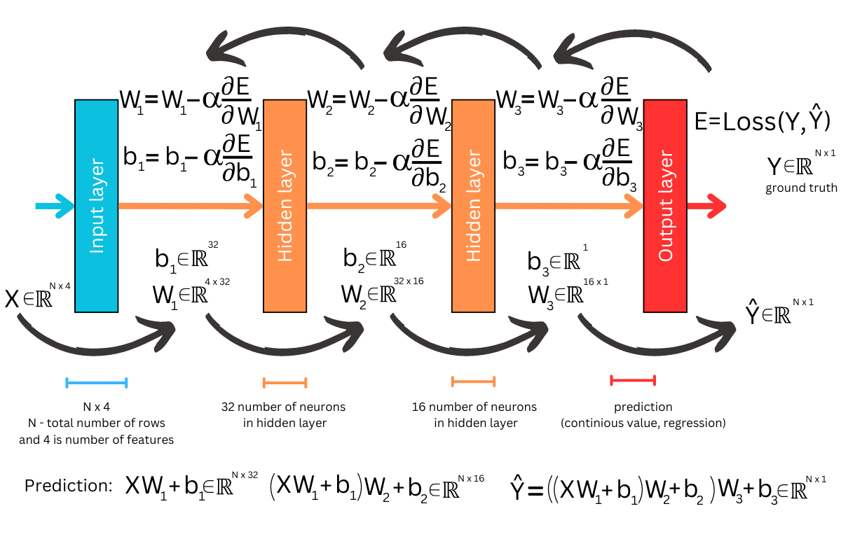
While focusing on the simplicity of neural network, it’s important to also mention the role of bias. Each neuron in an neural network includes a bias term in addition to its weights, which helps to shift the activation function to better fit the data. This addition of bias ensures that even if all input features are zero, the neuron can still contribute a non-zero output, enhancing the model’s flexibility and its ability to capture more complex patterns. Just like the weights, the bias terms are adjusted during the backpropagation phase to optimize the network’s performance, ensuring that both weights and biases are fine-tuned to minimize the loss function.

Although our introduction to neural network is brief and only scratches the surface, the main focus of this blog is different. To gain a deeper understanding of the internal mechanisms of neural networks and their mathematical foundations, readers are encouraged to familiarize themselves with basic concepts from calculus and linear algebra as a starting point.

Jumping into JAX

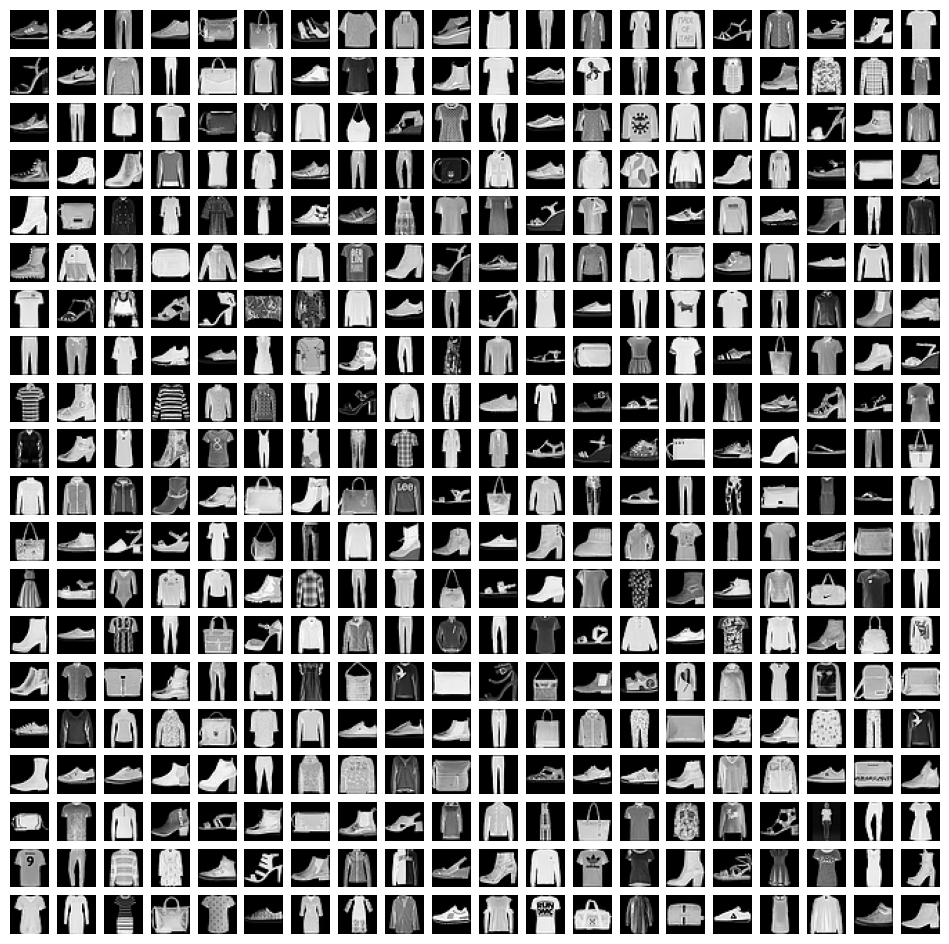
Let’s begin by implementing a neural network in JAX. Before diving into the core implementation, we’ll first create a few helper functions to handle dataset loading and batch iteration. For this demonstration, we’ll be using the Fashion MNIST dataset. This dataset contains 60,000 training images and 10,000 test images, distributed across 10 different clothing categories such as T-Shirts, Bags, Coats, and more. Each image is a grayscale, 28×28 pixel dimension, providing a standardized format for straightforward processing which means that we don’t need to do a lot of work in preprocessing phase.

import os
import gzip
import jax
import jax.numpy as jnp
import pandas as pd
import numpy as np
import matplotlib.pyplot as plt

from tqdm.notebook import tqdm
from functools import partial
from sklearn.metrics import accuracy_score, top_k_accuracy_score


def load_mnist_data(_path, _offset):
    
    with gzip.open(_path, "rb") as f:
        data = np.frombuffer(f.read(), np.uint8, offset=_offset)
        
    return data
    
    
    
class BatchGenerator:

    def __init__(self, X, Y, batch_size):
        self.X = X
        self.Y = Y
        self.batch_size = batch_size
        self.num_batches = (X.shape[0] - 1) // batch_size + 1

    def __iter__(self):
        for i in range(self.num_batches):
            start = i * self.batch_size
            end = start + self.batch_size

            yield self.X[start:end], self.Y[start:end]

The BatchGenerator, a helper class designed for iterating through the dataset in predefined batches. This class facilitates efficient handling of datasets by loading manageable chunks at a time, which is crucial for effective learning. Additionally, we utilize the load_mnist_data function, another essential tool that assists in loading the Fashion MNIST data from its binary format as provided in the repository. Together, these utilities enable us to optimize the learning process through batch iteration, a method proven to enhance learning efficiency by ensuring that our model gradually adjusts to the data without being overwhelmed by its volume.

DATASET_PATH = "<PATH_TO_DATASET_FILES>"
TRAIN_PATH, TEST_PATH = os.path.join(DATASET_PATH, "train-images-idx3-ubyte.gz"), os.path.join(DATASET_PATH, "t10k-images-idx3-ubyte.gz")
TRAIN_LABELS_PATH, TEST_LABELS_PATH = os.path.join(DATASET_PATH, "train-labels-idx1-ubyte.gz"), os.path.join(DATASET_PATH, "t10k-labels-idx1-ubyte.gz")


TRAIN_LABELS_NP = load_mnist_data(TRAIN_LABELS_PATH, 8)
TRAIN_DATA_NP = (load_mnist_data(TRAIN_PATH, 16).reshape(len(TRAIN_LABELS_NP), 784) / 255.0).astype(np.float32)

TEST_LABELS_NP = load_mnist_data(TEST_LABELS_PATH, 8)
TEST_DATA_NP = (load_mnist_data(TEST_PATH, 16).reshape(len(TEST_LABELS_NP), 784) / 255.0).astype(np.float32)


fig, ax = plt.subplots(20, 20, figsize=(12, 12))

for i in range(20):
    for j in range(20):
        ax[i, j].imshow(TRAIN_DATA_NP[np.random.randint(0, len(TRAIN_LABELS_NP), 1).item()].reshape(28, 28), cmap="gray")
        ax[i, j].axis("off")

        ax[i, j].set_xticks([])
        ax[i, j].set_yticks([])
        
plt.show()

Once the data is loaded from the files, it is stored in numpy arrays, allowing for easy manipulation. After loading, we convert each image into a 784-length vector (flattening the 28×28 pixel image). Each pixel value is then normalized by dividing by 255. This normalization step is crucial because it scales the pixel values to a range of 0 to 1, facilitating the learning process. Normalized data improves the efficiency of gradient descent by ensuring consistent scaling and variance across the dataset, which in turn enhances the model’s ability to find the optimal parameters and achieve minimal loss more effectively.

Neural network initialization

Now, let’s revisit Figure 4, which illustrates the matrix viewpoint of a neural network—the exact framework we aim to implement. Using JAX’s robust functions, you’ll see just how straightforward this process can be. Our first step involves defining a function to initialize random parameters that align with the specified layer configuration.

def init_mlp_params(layers_configuration: list[int], seed: int):
    key = jax.random.PRNGKey(seed)
    key, *subkeys = jax.random.split(key, len(layers_configuration))
    
    params = []
    for (i, units) in enumerate(layers_configuration[1:]):
        params.append((
            jax.random.normal(subkeys[i], (layers_configuration[i], layers_configuration[i + 1])), # W
            jax.random.normal(subkeys[i], (layers_configuration[i+1],))                            # b
        ))
    
    return params
    
    
_params = init_mlp_params([784, 32, 10], seed=42)

[
    {
        'W': p[0].shape,
        'b': p[1].shape
    } for p in _params
]
# [{'W': (784, 32), 'b': (32,)}, {'W': (32, 10), 'b': (10,)}]

Here it is, our first function in JAX for initializing the parameters of a neural network. The function, init_mlp_params, takes a list of integers as input, where each integer specifies the number of neurons in a corresponding layer of the network. For example, the input [784, 32, 10] indicates a neural network with three layers: the input layer with 784 features (corresponding to the input data dimensions), a hidden layer with 32 neurons, and an output layer with 10 neurons.

The function returns the weights W and biases b for each layer, organized as a list of tuples. In each tuple, the first element is the weight matrix W and the second element is the bias vector b. For instance, with our given input, the first weight matrix will have the dimensions 784×32 to match the input layer and the first hidden layer. This matrix transforms the input data matrix X (with dimensions Nx784, where N is the number of samples) into a matrix of dimensions Nx32. This transformation is part of the neural computation, where the matrix multiplication XW is followed by adding the bias term and applying an activation function. This structure is consistent with what we anticipated and is illustrated in Figure 4.

There is a important difference in the code from classical Numpy library and it is in working with random numbers which our function actually begins. In these lines of code, we begin by generating a primary random key using JAX’s pseudo-random number generator (PRNG) system, which is initialized with a specific seed. This key is crucial for ensuring reproducibility in experiments. The second line splits this primary key into multiple subkeys, with the number of subkeys matching the length of layers_configuration, which specifies the architecture of the neural network. Each subkey is intended for use in the random initialization of parameters for each respective layer in the network, helping maintain independence between the layers’ initial values. Then we starts with generating matrices from standard normal distribution using function jax.random.normal(…) using straight forward for-loop through list of integers and generating matrices with appropriate dimensions.

• jax.random.PRNGKey(seed)
  • Creates a pseudo-radnom number generator (PRNG) key given an integer seed
• jax.random.split(key, len(layers_configuration))
  • Split the PRNG key into as many new keys as there are layers in layers_configuration
  • Each resulting key is used to independently initialize the random weight matrices and bias vectors for each layer, ensuring unique random values across the network
• jax.random.normal(subkeys[i], (layers_configuration[i], layers_configuration[i + 1]))
  • Generate a normal distribution of random values using subkeys[i] for the specified layer
  • The shape of the generated matrix is determined by layers_configuration[i] (number of neurons in the current layer) and layers_configuration[i + 1] (number of neurons in the next layer), ensuring compatibility for matrix operations between layers
  • While this method initializes weights using a normal distribution, it is not the optimal approach for all neural network configurations; however, it is sufficient for initial experiments and demonstrations

Feedforward it

@jax.jit
def forward(params, inputs):
    activations = inputs
    *hidden_layers, output_layer = params
            
    for (W, b) in hidden_layers:        
        activations = jnp.dot(activations, W) + b
        activations = jax.nn.relu(activations)
        
    return jax.nn.softmax(jnp.dot(activations, output_layer[0]) + output_layer[1])

Feedforward phase of the neural network, which is a crucial method for making predictions. The feedforward process begins by taking the entire dataset or a batch of data, represented in matrix form. We then iterate through each layer of the network, applying the respective weight matrix (W) and bias vector (b) to the data. For each hidden layer, after the matrix multiplication and bias addition, an activation function is applied to introduce non-linearity and help the network learn complex patterns. In contrast, the output layer typically performs a linear combination of the inputs and weights, adding the bias term but not applying an activation function. This distinction is important as it allows the network to produce the final output values that are used for making predictions or classifications.

• jnp.dot(activations, W)
  • Calculate the dot product of the activations matrix and the weight matrix W, similar to using numpy.dot. This operation combines the input features linearly using the weights
• jax.nn.relu(activations)
  • Apply the ReLU function element-wise to the activations matrix to introduce non-linearity
  • ReLU(x) = max(0, x)
• jax.nn.softmax(jnp.dot(activations, output_layer[0]) + output_layer[1])
  • Apply the softmax function to the output layer results
  • This converts raw output values into probabilities for each class
  • Ensures all probabilities sum to one, making them directly interpretable
  • Softmax(x)_i = e^x_i / Σe^z_j

Backpropagation

@jax.jit
def make_safe_log(x):
    epsilon = 1e-12
    safe_x = jnp.where(x < epsilon, epsilon, x)
    
    return jnp.log(safe_x)


@jax.jit
def loss_fn(params, inputs, targets):
    targets_one_hot = jax.nn.one_hot(targets, 10)    
    preds = forward(params, inputs)
    
    result = -jnp.mean(jnp.sum(targets_one_hot * make_safe_log(preds), axis=1))
    return result


@jax.jit
def update(params, inputs, targets, lr=1e-3):
    loss_val, grads = jax.value_and_grad(loss_fn)(params, inputs, targets)
    return [(W - lr * dW, b - lr * db) for (W, b), (dW, db) in zip(params, grads)], loss_val

Now we advance to the final phase of neural network implementation: backpropagation. This phase leverages the predictions from the feedforward process, updating the weights across each layer to minimize the error. In this context, error refers to the discrepancy between the predicted outputs and the actual class labels. Given that we are addressing a classification task with ten labels, we utilize categorical cross-entropy loss, a standard choice for such scenarios.

To prepare for this, we convert class labels (ranging from 0 to 9) into one-hot vectors. Each one-hot vector is the same length as the number of classes, with a 1 at the position corresponding to the class label and 0s elsewhere. For example, the label ‘5‘ is represented as [0, 0, 0, 0, 0, 1, 0, 0, 0, 0], and the label ‘1‘ as [0, 1, 0, 0, 0, 0, 0, 0, 0, 0]. This conversion is efficiently handled by the JAX function jax.nn.one_hot.

Following this setup, we proceed with a typical training step: we call the forward(params, input) function to generate predictions and then compute the loss using the one-hot encoded targets. The actual loss computation and parameter updates are performed in the update(params, inputs, targets, lr=1e-3) function, which constitutes a single iteration of backpropagation. Each iteration calculates gradients for each weight matrix and bias vector, and updates them according to the gradient descent rule. An important parameter we haven’t previously mentioned is the learning rate (lr). This is a hyperparameter that must be defined before the learning process begins. The learning rate dictates the size of the steps taken towards the optimal point during the learning process, influencing how quickly or slowly the network learns. Through numerous iterations, this meticulously controlled process gradually enables the neural network to recognize patterns and improve its predictive accuracy.

JAX is equipped with excellent automatic differentiation (autodiff) system, which is a fundamental component of modern machine learning techniques. In JAX terminology, functions that perform automatic differentiation are referred to as transformations. Two such transformations are available for our use:

• jax.grad(…)
  • creates a function that evaluates the gradient of passed function
• jax.value_and_grad(…)
  • similar as jax.grad(…) just beside the gradient it returns value of function before transformation

def f(x):
    return x**2

f_grad = jax.grad(f)
f_grad(2.0)

# Array(4., dtype=float32, weak_type=True)

Like on example shown, calling jax.grad(…) and using it is pretty straightforward:

• define function
  • in our case it is single variable function, f(x)=x**2
  • derivative of this function is f'(x)=2x
• get gradient
  • f_grad is a function which evaluates f’ in given point a, f'(a)

def f(x, y):
    return jnp.sum((x - y)**2)
    
    
f_dx = jax.grad(f) # or jax.grad(f, argnums=0)
x = jnp.array([1.0, 2.0, 3.0])
y = jnp.array([2.0, 3.0, 4.0])

f_dx(x, y)
# Array([-2., -2., -2.], dtype=float32)


f_dxdy = jax.grad(f, argnums=(0, 1))
f_dxdy(x, y)
# (Array([-2., -2., -2.], dtype=float32), Array([2., 2., 2.], dtype=float32))


f_dy = jax.grad(f, argnums=1)
f_dy(x, y)
# Array([2., 2., 2.], dtype=float32)

What happens if a function involves multiple variables and we want to compute gradients for one or more of these variables? As demonstrated earlier, this can be easily managed in JAX using the argnums parameter, which specifies which variables should be considered for gradient computation (default value is 0):

• define function
  • in our case it is function with two variables, f(x, y) = sum((x-y)**2)) (remember when we talk about variables it may be scalars but as well vectors or event matrices)
  • derivatives of this function are
    • df/dx = 2(x-y)
    • df/dy = 2(x-y)(-1)
• get gradients
  • f_dx is a function which evaluates df/dx at point (x,y)
    • x=[1, 2, 3] and y=[2, 3, 4], df/dx = [2(1-2), 2*(2-3), 2*(3-4)] = [-2, -2, -2]
  • f_dy is a function which evaluates df/dy at point (x, y)
    • x=[1, 2, 3] and y=[2, 3, 4], df/dy=[2*(1-2)*(-1), 2*(2-3)*(-1), 2*(3-4)*(-1)] = [2, 2, 2]
  • f_dxdy is a function which evaluates df/dx and df/dy and return gradients
    • it will return something like ([-2, -2, -2], [2, 2, 2])

Now that we have access to powerful functions for gradient computation, the implementation of the update(…) function becomes quite straightforward. We simply use the loss function and call jax.value_and_grad(…) to compute gradients for all weight matrices and bias vectors. The structures that store parameters (params) and the gradients (grads) computed by JAX are structural identical (list of tuples), allowing us to iterate over them in the same manner to update the weights and biases.

Lets spin training

batch_size = 128
iterations = 500

np.random.seed(42)
indices = np.random.permutation(len(TRAIN_LABELS_NP))

train_indices = indices[:int(0.8 * len(TRAIN_LABELS_NP))]
val_indices = indices[int(0.8 * len(TRAIN_LABELS_NP)):]


train_batch_generator = BatchGenerator(TRAIN_DATA_NP[train_indices], TRAIN_LABELS_NP[train_indices], batch_size)
val_batch_generator = BatchGenerator(TRAIN_DATA_NP[val_indices], TRAIN_LABELS_NP[val_indices], batch_size)


with tqdm(total=iterations, desc='Training') as pbar:

    for _iter in range(iterations):            
        for batch_X, batch_Y in train_batch_generator:
            _params, loss_val = update(_params, batch_X, batch_Y, lr=1e-3)
            
        pbar.set_postfix({"val_loss": val_loss, "loss": train_loss})          
        pbar.update(1)

Now that we have all the ingredients in place, we can begin the training process of a neural network model using a dataset divided into training and validation sets. Initially, the batch size is set at 128, and the training is scheduled to run for 500 iterations. To ensure reproducibility, the dataset indices are shuffled using a random seed.

The data is then partitioned into training and validation sets, allocating 80% for training and the remaining 20% for validation. BatchGenerator objects are set up for both sets, configured to generate batches of data of the specified size.
During the training phase, employing a method known as stochastic gradient descent (SGD), the model undergoes the specified number of iterations. Each iteration processes the training data in batches. Within each batch, the update function is invoked to adjust the model’s parameters (_params), using the batch data (batch_X and batch_Y) and a learning rate of 0.001. However, there is no guarantee that the loss function will achieve optimal results during training. The effectiveness of the training process depends on numerous factors, including the nature of the data, the characteristics of the problem being addressed, and the settings of hyperparameters.

Before we proceed to examine the loss and accuracy results, it’s important to note that we began with Numpy arrays and did not perform any explicit conversion to jax.Array, the primary array type used by JAX. Thanks to Python’s duck-typing system, JAX arrays and Numpy arrays can often be used interchangeably in many contexts. This compatibility allows us to use Numpy arrays in function calls within JAX operations without concerns about compatibility issues.

Evaluation

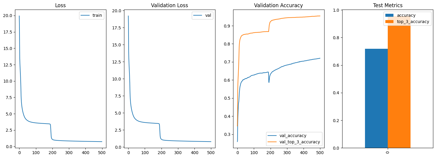
Let’s review the results. Surprisingly, the outcomes are quite favorable, considering that the neural network was assembled without experimenting with different layer configurations or fine-tuning hyperparameters. During the training phase, the loss stabilized at around 0.74, while the validation loss was slightly higher at around 0.78. The model achieved an accuracy of 71% (0.71) on the test data, which it had never seen during training. Moreover, the top-3 accuracy reached an 95% (0.95). Pretty solid results, right? Why not spin up the model yourself and see if you can tweak it to get even better numbers? Give it a shot!

Now that our model is trained, we can use it to make predictions on any image that fits the input layer. However, for our purposes, it’s sufficient to use the test dataset that’s already available. This dataset includes images that were not seen during the training phase, allowing us to verify the model’s accuracy after training is complete.

@jax.jit
def predict(params, inputs):
    return jnp.argmax(forward(params, inputs), axis=1)


fig, ax = plt.subplots(5, 5, figsize=(20, 18))

for i in range(5):
    for j in range(5):
        idx = np.random.randint(0, len(TEST_LABELS_NP), 1).item()
        ax[i, j].imshow(TEST_DATA_NP[idx].reshape(28, 28), cmap="gray")
        ax[i, j].set_title(f"Predicted: {predict(_params, TEST_DATA_NP[idx:idx+1]).item()}\nTrue: {TEST_LABELS_NP[idx]}")
        ax[i, j].axis("off")
        
        # make margin between images for better visualization
        ax[i, j].set_xticks([])
        ax[i, j].set_yticks([])
        
        # text color of title make to be blue
        ax[i, j].title.set_color('blue')
                    
plt.show()

@jax.jit
def predict_proba(params, inputs):
    return forward(params, inputs)


@jax.jit
def predict(params, inputs):
    return jnp.argmax(forward(params, inputs), axis=1)
    
    
    
pd.DataFrame({
    "accuracy": [accuracy_score(TEST_LABELS_NP, predict(_params, TEST_DATA_NP))],
    "top_3_accuracy": [top_k_accuracy_score(TEST_LABELS_NP, predict_proba(_params, TEST_DATA_NP), k=3)]
})

#{
#  'accuracy': 00.7187 Name: accuracy,
#  dtype: float64,
#  'top_3_accuracy': 00.954 Name: top_3_accuracy,
#  dtype: float64
#}

Summary

In this exploration, we’ve seen firsthand how JAX is an excellent library for working with machine learning models, offering robust tools for operations like automatic differentiation and efficient numerical computations. However, the neural network we implemented, while functional, is not the most optimal for our specific use case. A Convolutional Neural Network (CNN) would likely achieve much better accuracy due to its suitability for handling image data. Towards the end, we addressed aspects of numerical stability in our code, such as implementing a make_safe_log function to prevent issues like NaN values in loss calculations. For example, if you replace make_safe_log(x) with jnp.log(x) in the loss_fn(…), the loss function might return NaN after a few iterations. This occurs because jnp.log(x) can produce NaN if x is zero or very close to zero, demonstrating the importance of maintaining numerical stability during model training. You can find the complete code for this project at the link.